C. GAY, F. ESTRADA and C. CONDE
Centro de Ciencias de la Atmósfera, Universidad Nacional Autónoma de México,
México, D. F. 04510 México
Corresponding author: F. Estrada; e–mail: feporrua@atmosfera.unam.mx
Received May 16, 2006; accepted August 25, 2006
]]>RESUMEN
La práctica común de utilizar submuestras de periodos de 30 años de datos climatológicos para describir las condiciones pasadas, presentes y futuras ha sido ampliamente aplicada, en muchos casos sin considerar las propiedades de la serie de tiempo analizada. Este trabajo muestra que esta práctica puede llevar, tanto a un uso ineficiente de la información contenida en los datos, como a una caracterización imprecisa de las condiciones climáticas actuales, y en particular de las futuras, debido a que los parámetros son función del tiempo y del tamaño de la submuestra. Más aún, este enfoque puede llevar a la detección de cambios espurios en los parámetros de la distribución de la variable analizada. En este trabajo se utiliza el análisis de series de tiempo de las temperaturas mensuales observadas en Veracruz, México, para ilustrar el hecho de que estas técnicas permiten realizar una mejor descripción de la media y variabilidad de las series, lo que a su vez permite (dependiendo de la clase de proceso) restringir la incertidumbre del pronóstico, y por lo tanto ofrecer una mejor estimación del riesgo presente y futuro de observar valores fuera de un rango de tolerancia dado. Los resultados presentados en este trabajo muestran que, si bien se encuentra una tendencia significativa en las temperaturas, aportando posible evidencia observada de cambio climático en la región, no existe ninguna que apoye cambios en la variabilidad de dichas series, y por lo tanto tampoco existe ninguna evidencia observada a favor de que la variabilidad de la temperatura mensual aumentará o disminuirá en el futuro. Esto es, si el cambio climático ya está ocurriendo, se ha manifestado como un cambio en la media de estos procesos y no ha afectado otros momentos de sus distribuciones (procesos no–estacionarios homogéneos). El Magicc–Scengen, un programa útil para la construcción de escenarios de cambio climático, utiliza submuestras de 20 años para estimar la variabilidad futura del clima. Para propósitos de comparación, se construyeron posibles funciones de densidad futuras siguiendo dos enfoques distintos: el primero utilizando únicamente las salidas del Magicc–Scengen, y el segundo usando una combinación de esta información y del análisis de series de tiempo. Se muestra que las estimaciones basadas en submuestras pueden llevar a una estimación imprecisa de los impactos potenciales de la variabilidad climática presente y de los escenarios de cambio climático en términos de las probabilidades de obtener valores fuera de un rango de tolerancia dado.
ABSTRACT
The common practice of using 30–year sub–samples of climatological data for describing past, present and future conditions has been widely applied, in many cases without considering the properties of the time series analyzed. This paper shows that this practice can lead to an inefficient use of the information contained in the data and to an inaccurate characterization of present, and especially future, climatological conditions because parameters are time and sub–sample size dependent. Furthermore, this approach can lead to the detection of spurious changes in distribution parameters. The time series analysis of observed monthly temperature in Veracruz, México, is used to illustrate the fact that these techniques permit to make a better description of the mean and variability of the series, which in turn allows (depending on the class of process) to restrain uncertainty of forecasts, and therefore provides a better estimation of present and future risk of observing values outside a given coping range. Results presented in this paper show that, although a significant trend is found in the temperatures, giving possible evidence of observed climate change in the region, there is no evidence to support changes in the variability of the series and therefore there is neither observed evidence to support that monthly temperature variability will increase (or decrease) in the future. That is, if climate change is already occurring, it has manifested itself as a change–in–the–mean of these processes and has not affected other moments of their distributions (homogeneous non–stationary processes). The Magicc–Scengen, a software useful for constructing climate change scenarios, uses 20–year sub–samples to estimate future climate variability. For comparison purposes, possible future probability density functions are constructed following two different approaches: one, using solely the Magicc–Scengen output, and another one using a combination of this information and the time series analysis. It is shown that sub–sample estimations can lead to an inaccurate estimation of the potential impacts of present climate variability and of climate change scenarios in terms of the probabilities of obtaining values outside a given coping range.
1. Introduction
Observed monthly temperature series are analyzed using time series techniques to infer the underlying data generating process and whether or not it has changed over time. The analyses performed reveal important results regarding monthly temperature mean and variability that have relevant implications for describing current climatologic conditions and for forecasting purposes. In earlier works (Gay et al., 2006; Gay et al., 2004; Conde et al., 2005), the authors have studied the potential impacts of climate change in agriculture, in particular for coffee production in Veracruz, México. The assessment of the potential risk that climate change represents for coffee producers in the region motivated the analysis presented herein.
The recommendations of the World Meteorological Organization (WMO) for using periods of at least 30 years to describe climate conditions have been extensively used, in most cases without considering the time series properties of the observed variables*. This approach is intended to offer an easy way to describe past, present and future climate, and for some applications it can provide an acceptable approximation. Nevertheless, for risk, vulnerability and impact assessments, among others, a more precise approach is required. An example of erroneous application of this approach can be found in government agencies and insurance companies in México, which usually use this 30 years description for assessing the probabilities of observing climate variables outside normal conditions, and for determining if an event was unusual enough to warrant insurance claims. In many cases this has resulted in controversies and mistakes (Gay et al., 2004b). This practice has also been extended for describing future climate through results from General Circulation Models (GCM) runs based on different emission scenarios and models (Ruosteenoja et al., 2003; Wigley, 2003), and in the widely used Magicc–Scengen software. This approach is not adequate if the series have a stochastic or deterministic trend and can produce spurious changes in distribution parameters.
]]> In the second section of this paper it is shown how this common practice can lead to an inefficient use of the information contained in the data and to an inaccurate characterization of present, and especially future, climatological conditions because parameters are time and sub–sample size dependent. Moreover, if the process is stationary, why to limit sample size to 30 years if more data is available for obtaining a better estimation of the relevant distribution parameters?; and if the process is known to be non–stationary, why use standard statistical techniques that require stationarity? Let us note that, if the process is non–stationary, ergodic properties do not hold either.Results in Section 3 show that, although for most months in the region there is evidence of what could be a signal of climate change (expressed in terms of a statistically significant linear trend), the series are otherwise stationary processes (trend–stationary). That is, if climate change is already occurring, it has manifested itself as a change–in–the–mean of these processes and has not affected other moments of their distributions (homogeneous non–stationary processes (Guerrero, 2003)).
A large number of studies on climate change have focused on searching for human induced changes in climate variables that could be expressed, for example, through statistically significant trends (Vogelsang and Franses, 2001; Bloomfield, 1992; Zheng and Basher, 1999; Galbraith and Green, 1992; Woodward and Gray, 1993, 1995), and cointegration between series of atmospheric concentrations of greenhouse gases and temperature (Stern and Kaufmann, 1997, 1999; Kaufmann and Stern, 1997). Many others have shed important light about the frequency of occurrence of extreme events (analyses of maximum values, or values exceeding a threshold value), but in most cases there is too little data (and of too poor quality) to assess observed changes in their frequency. One of the most unsettled questions regarding climate change is how, and if, it will affect climate variability, and especially the frequency and intensity of extreme events. As shown in Section 3, time series techniques permit to make a better description of the mean and variability of the series, which in turn allows (depending on the class of process) to limit uncertainty of forecasts and thereby giving better estimation of present and future risk of observing values outside a given coping range. This information can be used for better assessing present risk in activities or sectors of interest and for generating future hybrid scenarios (probability distributions) using GCM outputs and time series analysis.
Results show that, although a significant trend is found in most cases, giving possible evidence of observed climate change in the region, there is no evidence to support changes in the variability of the series and therefore there is neither observed evidence to support that monthly temperature variability will increase or decrease in the future. This is in clear contrast with the scenarios that can be constructed using the Magicc–Scengen, given that it projects the standard deviation of temperature to be a function of time. Two main issues are discussed regarding this topic: the projected increase–decrease in variability could be produced by the use of an erroneous approach (the use of a fixed number of years to describe temperature) and; although in some senses an increase–decrease in variability could imply a larger–lesser threat, it is shown that it could lead to under–overestimating the potential impacts of climate change in terms of the probabilities of having values outside a given coping range. Possible future probability density functions are constructed using the mean and standard deviation, provided by the Magicc–Scengen software for the region, and compared to the ones obtained constructing a hybrid model that uses the predicted mean values obtained from the ECHAM (European Centre Hamburg Model) and the statistical information extracted from time series analysis.
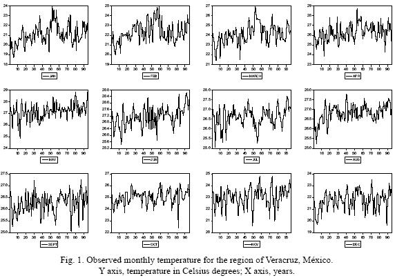
The data for the monthly mean values from 1901 to 1995 were obtained from the IPCC Data Distribution Center (http://ipcc–ddc.cru.uea.ac.uk/java/time_series.html) for the selected region, that is located between 98–93° N and 22–17° W. Figure 1 shows a time series plot of monthly mean values for 1901 to 1995.
2. Common practices for describing a supposedly time–homogeneous process
An adequate statistical analysis of observed climate variables and of GCM–runs is of prime importance when assessing the potential impacts on different human and natural systems due to climate change. Risk assessment, policy making, and adaptation strategies critically depend on this input and on how well uncertainty can be addressed and reduced using all available information.
]]> According to the IPCC (http://www.grida.no/climate/ipcc_tar/wg1/518.htm, "climate in a narrow sense is usually defined as the 'average weather', or more rigorously, as the statistical description in terms of the mean and variability of relevant quantities over a period of time ranging from months to thousands or millions of years. The classical period is 30 years, as defined by the World Meteorological Organization (WMO, 1983)". This approach has been widely used to compare climate from different periods of 30 years and for comparing present and future climate variability implied by climate change scenarios. As will be shown, this approach is not consistent: in order to apply standard statistics, the series needs to be time–homogeneous (stationary), and if the process is time–homogeneous, limiting the sample size to 30 years leads to an inefficient estimation of true distribution parameters.The Magicc–Scengen provides changes in climate variability, where "variability is defined by the inter–annual standard deviation over 20–year intervals" (Wigley, 2003). Furthermore, "variability changes are expressed as ratios, i.e. future standard deviation divided by initial (present–day) standard deviation minus 1, expressed as a percentage. A zero value therefore represents no change, while positive or negative values represent, respectively, increases or decreases in variability". Climate change, by definition, implies that climate variables will not be a time–homogeneous process (i.e. the time variable plays an important role given that distribution parameters will change as time goes by) and thus computing standard measures of variability for this type of process will produce erroneous results.
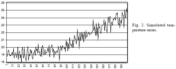
To illustrate this, consider the following model:
Tt = α + βt + εt
where Tt is a simulated temperature value for time t, a is a constant that in this case takes the value of 19 °C, >β is a non–constant parameter that takes the values of zero from t = 0 to t = 29; 0.015 from t = 30 to t = 89 and; 0.055 when t > 90; and is et a normally distributed random variable with mean zero and standard deviation of 0.6 °C. The mean and variance of this process are:
E (Tt) = E (α + βt + εt) = α + βt
Var (Tt) = Var (α + βt + εt) = σ2ε = 0.36
Cov (εtεt–1) = 0 for t ≠ t'
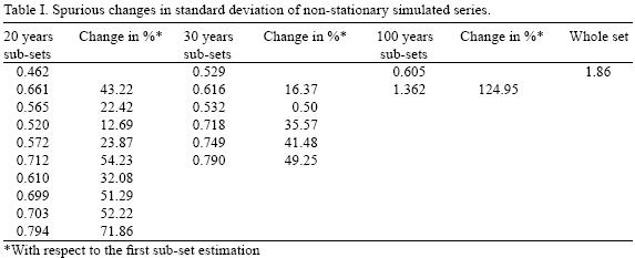
That is, by construction, the mean of the process is a function of time, but its variance is constant. A realization of this process for a sample length of T = 200 is shown in Figure 2. Table I shows the standard deviation of this process calculated for three different sub–sample sizes: 20 as chosen by the Magicc–Scengen, 30 as is commonly done and 100 (half sample). It is important to notice that when calculating the change in variability, the standard deviation of the process is shown to increase up to a 124.95%, depending on the sub–sample size used for the estimation. Using the whole sample leads to a more than three times larger variability than its true value.
]]>
That is, although by construction the standard deviation of the process is known to be constant, we are led to believe that the process variability is increasing due to the non–stationarity produced by a trend. In summary, if the process is time–homogeneous (stationary), restricting sample size will only lead to an inefficient use of data and imprecise parameter estimations, and when the process is non–stationary even if the sample size is restricted, estimations are very likely to be misleading.
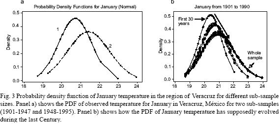
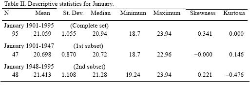
The same can be shown using a "real" observed temperature series. Figure 3a shows the probability density function (PDF) of the observed temperature for January in Veracruz, México, for two sub–samples (1901–1947 and 1948–1995). The PDF for each sub–sample apparently assigns probabilities very differently, such that it is clear that the second sub–sample has fatter tails, greater dispersion and a wider range. Furthermore, Figure 3b presents how the PDF of January temperature has supposedly evolved during the last century. This would imply that the variability and range of extreme events increased notably in the last part of the 20th century. Table II shows the descriptive statistics for January (see also Figure 1 for a plot of the series) and how distribution moments have been supposedly evolving through time. Nevertheless, these results are clearly as inconsistent as in the simulation example shown before, because if the distribution parameters are not constant, then the process is non–stationary and therefore the standard statistical procedures that were applied are no longer valid.
]]> 3. Time series approach for assessing changes in temperature distribution
Strict stationarity indicates that all joint probability distribution of the random variables that constitute the process underlying a time series does not change in time. That is, all distribution parameters remain constant. Given that strict stationarity is difficult to obey and even to verify in practice, second order (also called wide–sense, weak or covariance) stationarity is commonly used, and if the variables underlying the series follow a normal distribution, strict and second order stationarity are equivalent (Maddala and Kim, 1998). Weak or covariance stationarity implies that no changes in the standard deviation are present, the mean does not change, and that the autocovariances depend on the lag length but not on absolute time. Examples of this class of processes are white noise and autoregressive (AR) and moving average processes (MA) and auto regressive moving average (ARMA).
The most common examples of non–stationary processes are trend–stationary and difference–stationary (Nelson and Plosser, 1982), and it is of special interest to distinguish between them because that distinction determines the statistical properties of a series (in this case the implications about the series variability are of special interest) and allows to infer the proper transformation needed to apply standard statistical procedures.
A trend stationary process is composed of a deterministic component with the addition of a stochastic process (white noise, AR, MA, ARMA) that satisfies the stationarity conditions. A simple example of this class of process is an AR equation of the form:
xt = α + βt + ρxt–1 + et (1)
where α is a constant, | ρ | < 1, et ~ i.i.d (0, σ2)** is a white noise process, that could also be extended to an ARMA process that satisfies the stationarity and invertibility conditions, and βt is a deterministic trend. (For a detailed explanation on these conditions see Guerrero, 2003; Enders, 2003). This process is mainly dominated by its deterministic component and therefore has a tendency to revert to its trend. That is, variations are transitory and do not change the long run path of the series (Enders, 2003). The mean of this process E (xt) = α + βt is not constant but can be known for any t+ s. The assumption of a deterministic trend is not as restrictive for climate variables if we consider that it can be any function of time, although for the objectives of this paper we will consider the simplest case of a linear trend. One of the most important characteristics of the trend stationary process is that its variance Var (xt) is constant. This has important implications for the variability of a series and it means that the forecast error is bounded (Greene, 1999; Maddala and Kim, 1998).
On the other hand, a series is said to be integrated or difference–stationary if it contains a stochastic trend. If a series is stationary in levels is said to be I (0), if it has to be differenced once is I (1), and it is I (2) if it has to be differenced twice to achieve stationarity. The following equation of a random walk is a common example of an I (1) type of process:
yt = yt–1 + et (2)
or
Δyt = et
]]> where Δ = (1 – L) is the difference operator, et ~ i.i.d (0, σ2) is a white noise process that could also be an ARMA process satisfying the stationarity and invertibility conditions. This model is a special case of an AR (1) process (when the coefficient of the autoregressive term is equal to one) and it is stochastic in nature, as can be shown if the difference equation (2) is solved: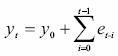
where y0 is the initial condition and

is a stochastic trend, a hardly predictable but systematic variation (Maddala and Kim, 1998), consisting in the sum of the stationary error term. Assuming the initial condition is zero, the mean of the process is zero E (yt) = E (et) = 0 and its variance increases with time Var (yt) = E (v2t) = tc2e and diverges as t  ∞ (Hatanaka, 1996). A generalization of equation (2) is a random walk with a drift (a constant term):
yt = β + yt–1 + et (3)
or
Δyt = β + et
The solution of this difference equation is
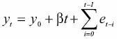

is a stochastic trend. In this case the variance of the process is Var (yt) = E (v2t) = tσ2e the same than in the case of a pure random walk, but the mean E (yt) = βt is no longer constant. It is important to notice that the differences between difference–stationary and trend–stationary arise from the presence of a stochastic trend, not from a deterministic trend.
As shown before, a difference–stationary process implies that its variance is a function of time and therefore the forecast error is not bounded and increases as the period to be forecasted is extended. Although both classes of processes have several interesting implications for climate variables, in this paper we will focus in the behavior of their variances. Trend–stationary and difference–stationary have important implications for how variability of a climate variable can be expected to be in future, and of the predictability of the series.
It is also important to notice, for statistical purposes, that these processes require different detrending methods to achieve stationarity and if they are misidentified, tests results and inferences can be misleading. A wide variety of formal tests to determine the order of integration of a series have been developed (for a survey see Stock, 1994). Here, two of the most common tests are considered: the Augmented Dickey–Fuller (ADF) (Dickey and Fuller, 1979; Said and Dickey, 1984), and the Phillips–Perron (PP) tests (Phillips and Perron, 1988).
The ADF test is based on testing the null of a unit root (a = 1) on the following models
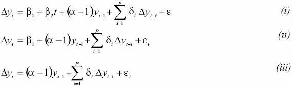
where βt is a linear trend, the lagged differences of yt are included to correct for autocorrelation (parametrically) and is a white noise error term. The upper bound for the lag length was determined using kmax = int (12 * (f/lOOVi)) (Hayashi, 2000) and the appropriate number of autoregressive terms was selected through minimizing the Akaike Information Criteria (Akaike, 1973).
Under the null of a unit root the distribution of the ordinary least squares (OLS) estimators is nonstandard and follows a Wiener process. In this case the t–statistics are no longer valid and the correct critical values have been tabulated (Dickey and Fuller, 1979; Phillips and Perron, 1998; MacKinnon, 1996). The null of models are pure unit root (i), unit root plus a drift (ii) and unit root plus a drift and a trend (iii). Under the alternative hypothesis the series is (i) trend–stationary, (ii) stationary around a constant, and (iii) stationary around zero.
The difference between the ADF and the PP tests is that the latter does not include lagged differences in equations i to iii, and corrects autocorrelation nonparametrically using the Barttlet kernel spectral estimator and the Newey–West automatic bandwidth selection.
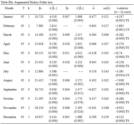
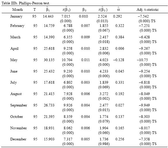
]]> The selection of the appropriate deterministic regressors to be included in both tests is of crucial importance because tests statistics depend on which regressors are included and because the power of the test (i.e. the ability of the test to reject the null when is false) is greatly affected. The procedure used to test for a unit root was that proposed by Dolado, Jenkinson and Sosvilla–Rivero, and showed in Enders (2003). As stated in Enders (2003) "the key problem is that the tests for unit root are conditional on the presence of the deterministic regressors and the tests for the presence of deterministic regressors are conditional on the presence of a unit root".Results of these tests are reported in Tables IIIa and IIIb. Results show that for all temperature series the null hypothesis of a unit root can be rejected at least at 95% confidence levels (except in the case of February for which the null can be rejected only at 90% by the Dickey–Fuller test) in favor of trend–stationarity (constant stationary in the case of February and July according to the ADF test). Therefore, the non–stationarity shown by the series can be considered to be the product of a changing mean, but a constant variance. That is, if the presence of a trend is interpreted as a sign of climate change, this process has shown to be a change–in–mean (homogeneous non–stationarity) and climate variability can be thought to be time invariant.
4. Projections of monthly temperature for 2050 and 2100
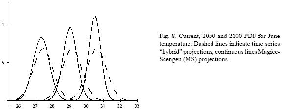
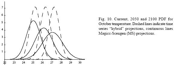
The main objective of this section is to obtain a model for the data generating process for the temperature series of a representative month of each season as well as to construct and compare future temperature PDF. The four months chosen are: January (winter), April (spring), June (summer) and October (fall).
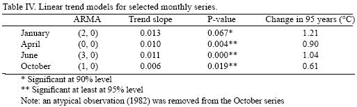
Table IV shows the time series models proposed for each of the selected months. June can be modeled as a trend–stationary autorregresive process of order three, January as a trend–stationary of order two, October as a trend–stationary first order autoregressive process, and April as a trend–stationary white noise process. Two important conclusions can be drawn from the misspecification tests (Table V): models are statistically adequate and therefore can be thought to be a correct representation of the data generating process, and the error terms are homoskedastic***. Two different heteroskedasticity tests were employed: one for unknown general forms of heteroskedasticity (White test) and one for autoregressive conditional heteroskedasticity (ARCH). Tests results show that, the variances of the error terms are homoskedastic and there is no volatility. It is also important to note that the null hypothesis of normally distributed errors cannot be rejected. For each of these temperature series a significant trend was found, ranging from 0.006 to 0.012; that is, an increase of 0.61 to 1.21 °C in the 95 years period of study. In summary, the data generating processes of these temperatures consist of a deterministic forcing component in the form of a linear trend (conditional mean) plus a normally distributed stationary processes (temperature variations) around this trend.
]]>
The variances and conditional means of these processes are of interest for developing current and future temperature PDF. Consider the general form of an autoregressive equation of orderp with a linear trend Yt = α + βt + ut, where
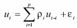
Its conditional mean and variance can be calculated as follows:
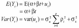
Table VI compares the estimated values of mean and standard deviation using time series and the 1961–1990 period as suggested by the WMO and the IPCC. It is important to notice that the estimations of mean are consistently lower using the 30 years period than those obtained with the conditional mean, while the differences in standard deviations range from –17.38 to +35.36%. That is, even for observed "current" climatologic conditions both methods give a dissimilar description, which in turn, would lead to differences in the estimations of present climatic risk for human or ecological systems. As stated in Section 1, the recommendations of WMO and IPCC (used by Magicc–Scengen, and others) can lead to poor estimations of the distribution's parameters and misleading risk estimations.
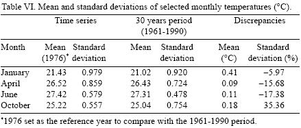
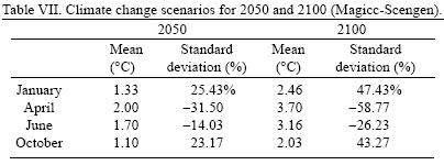
Table VII shows the climate change scenarios for 2050 and 2100 constructed using the Magicc–Scengen software. The ECHAM 498 model and the B2–MES emission scenario were chosen and the reference year was set to 1976 to compare with the 1961–1990 period. The range of changes in mean temperature goes from 1.1 to 2 °C for year 2050 and from 2.03 to 3.7 °C in 2100 depending on the month. On the other hand, predictions about the evolution of the standard deviation of temperature indicate that, for January, temperature variability could increase as much as 25% in 2050 and almost 50% in 2100 in comparison with current variability. For April, predictions of future variability imply a rather different evolution to a much less variable temperature: for 2050 it would decrease one third of its current value and for 2100 almost 60%.
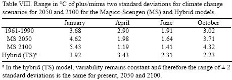
To illustrate what can be expected of such changes in variability, consider the interval centered in zero and plus/minus two standard deviations («95 % of the probability mass in a normal distribution). Table VIII shows the range in °C for the plus/minus two standard deviations for current (time series and 30 years average) and 2050 and 2100 climate change scenarios for the Magicc Scengen (MS) output and for the time series (TS) results. Comparing the ranges obtained from the two models, it can be seen that for current conditions the range from the 30 years average can be as 35% larger and 17% smaller than the time series range, depending on the month. These differences increase for future scenarios, such that for 2050 and 2100 the 30 years average can be as much as 67 and 94% larger and 42 and 65% smaller (respectively) in comparison with the time series estimation. For 2050, temperature variability within this range spans up to 4.62 °C and for 2100 it would reach 5.43 °C. A similar situation occurs for October's temperature. In contrast, April's and June's variability would be importantly reduced leading to an almost constant value with a range of 1.2 °C (for activities where the change in mean temperature are outside their coping ranges, an almost constant temperature could be very determinant for their viability). This has important implications for assessing the potential impacts of climate change for human and natural systems, and it is clear that for most current systems in the region it would be very difficult to cope with these types of changes in variability and in mean. Recent studies (Gay et al., 2006; Gay et al. 2004; Conde et al., 2005) show that some agricultural activities in the region can be very sensitive to changes in climate variability.
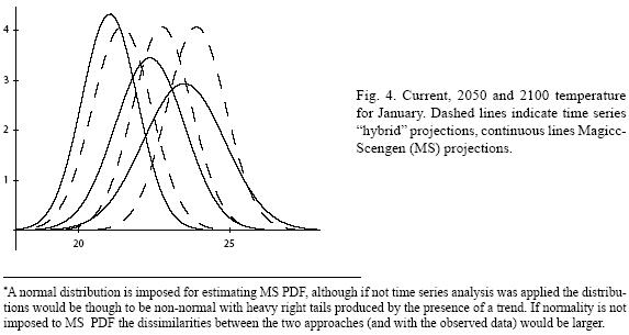
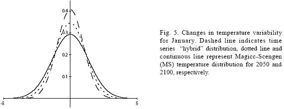
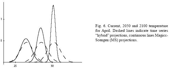
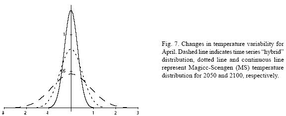
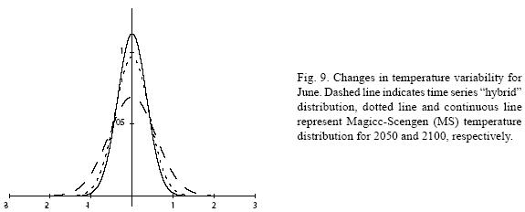
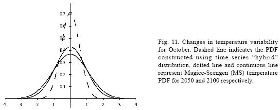
Figures 4 to 11 (Fugures 4, 5, 6, 7, 8, 9, 10, 11) show the PDF for current conditions and for climate change scenarios in 2050 and 2100****. The first figure for each month shows the evolution of the corresponding temperature PDF, while the second figure illustrates the changes in the variability. The PDF for April's and June's temperatures reveal that a reduction in variability can be more risky and produce greater potential impacts than an increase. Consider a given system that is well adapted to current temperatures. For 2050, and especially for 2100, such a system will face a completely different climate, given that probability densities assign completely different probabilities to temperature values (PDF span on almost completely different ranges and do not overlap). In addition, it is important to notice that for April and June the tails are much lighter for the case of MS scenarios than for the hybrid, leading to an underestimation of the occurrence of extreme events and their associated risk. For January and October the opposite situation occurs. As a result of the increase in the standard deviation, MS PDF overlap more than the ones obtained with the hybrid model. This assigns a higher probability to temperature values shown in current conditions for 2050 and 2100 scenarios, which in turn underestimates the potential impacts for a given activity that is well adapted to current conditions. On the other hand, the occurrence of extreme events from the right side of the temperatures' PDF is highly overestimated. In summary, projections that do not consider the time series properties of climate variables can be misleading for risk management and decision making.
For illustrative purposes, let's suppose that most of human and natural systems in the region are well adapted to the 1976 mean (that is, the time series equivalent for the 1961–1990 mean) plus/ minus 1.5 standard deviations (TS). Table IX shows the current, 2050 and 2100 probabilities for the fixed coping range. It is important to notice that even if climate variability does not increase (or even if it decreases), the frequency and magnitude of extreme values with respect to a fixed coping range increases because of the change in the mean of the distribution. In all cases, the probability of values below (P (X < μ – 1.5σ)) and within (P (μ – 1.5σ < X < μ +1.5σ)) the coping range decreases rather rapidly, especially in the representative months of spring and summer. All this probability is accumulated in the right side of the distribution, which represents an important raise in the occurrence and magnitude of extremely hot values for the systems that were well adapted for the previous climate. In fact, for April and June, systems that were adapted to the mean and plus/minus 1.5 standard deviations will be in 2100 completely outside their coping range.
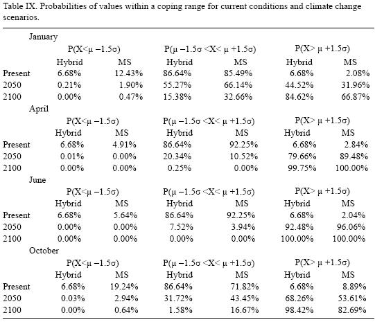
It is important to notice how the spurious changes in temperature variability (standard deviation), caused by not considering the stochastic properties of the time series, could lead to a poor estimation of present and future climate risk. Even for current conditions, if the recommendations of using 30 years sub–samples are applied, the occurrence of extreme***** cold temperature values for January and October are two and three times higher than the time series estimations. On the other hand the current probabilities of extremely high temperature values are underestimated for all months with the exception of October. The probability scenarios obtained with MS projections show that for the months for which their variability is expected to increase (January and October), the occurrence of extremely high temperature values (P (X μ +1.5σ)) is underestimated, while for the months for which its variability is expected to decrease (April and June) the opposite occurs. For the interval defined as the coping range P (μ – 1.5σ< X < μ+1.5σ) the MS projections overestimate the probabilities for January and October and for April and June the probabilities are underestimated. In all cases the probabilities of values below P (X < μ – 1.5σ) tend to zero as we approach year 2100.
5. Conclusions
]]> As stated by the WMO (1983), the most important applications of climatology and meteorology are: 1) Determination of the times of year which, on average, are favourable or unfavourable for the activities in question (that is economic activities); 2) Calculation of the probability to be assigned to the critical natural conditions beyond which the activity is impossible; 3) Examination of the action to be taken in order that the activity can be continued all the year round; 4) The development of strategies enabling those activities which are possible during most of the year, to be performed at minimum cost.In this paper it is shown how the common practice of using periods of 30 years for describing climate conditions (without considering the underlying stochastic properties of the process) can lead to poor estimation of statistical measures in the best case or to detecting spurious changes in distribution parameters that can be mistaken with manifestations of climate change. This, in turn, would not permit an adequate assessment of climate risk and the applications of climatology and meteorology mentioned above cannot be properly accomplished. If the series are believed to be stationary, limiting the sample size to 30 years provides an inefficient estimation; and if series are non–stationary, even if the sample size is restricted, estimations are very likely to be misleading.
The time series analysis of observed temperature series in the region of Veracruz, Mexico, reveals that monthly temperature series in the region can be considered as stationary around a linear trend (or in some cases a constant). It is relevant to take notice that, although the presence of a significant trend can be interpreted as a manifestation of climate change, the variance of the processes has remained constant. That is, climate change in the region has manifested itself as a change–in–mean phenomenon that has not altered the processes' variability.
The Magicc–Scengen software is a very useful tool for generating climate change scenarios and has been widely used in the assessment of its potential impacts, systems' vulnerability and as an input for developing adaptation strategies. The new version of this software provides scenarios for future climate variability, a very important variable for assessing potential impacts and vulnerability of a given system or activity. Nevertheless, the definition employed for determining the changes in climate variability is based on calculating the standard deviation in sub–samples of 20 years and does not take into account the time series properties of the underlying stochastic processes. Climate change and climate change scenarios imply, by definition, non–stationary processes and therefore standard statistical measures such as the standard deviation are affected and results are misleading. As an example, PDF constructed using MS outputs (mean and standard deviation) and from a hybrid model that combines MS change in mean and the information obtained from the time series analysis are compared. It is shown that both models provide different evolutions of temperature distributions. The two PDF obtained with these methods have different ranges of temperature values and assign dissimilar probabilities to them. MS estimations lead to under– and overestimating potential risks for a given activity or system in comparison with the hybrid model.
References
Akaike H., 1974. Anew look at the statistical model identification IEEE Transactions on Automatic Control, AC–19, 716–723. [ Links ]
Bloomfield P., 1992. Trend in global temperature. Clim. Change 21, 1–16. [ Links ]
Conde C., M. Vinocur, C. Gay, R. Seiler and F. Estrada, 2005. Climatic threat spaces as a tool to assess current and future climatic risk in México and Argentina. Two case studies. In: AIACC Synthesis of Vulnerability to Climate Change in the Developing World (..., Eds.) (In review). [ Links ]
Dickey D. A. and W. A. Fuller, 1979. Distribution of the estimators for autoregressive time series with a unit root, J. Amer. Statist. Assoc. 74, 427–431. [ Links ]
Enders W., 2003. Applied econometric time series. 2nd. ed., Wiley, New York, 480 pp. [ Links ]
Galbraith J. and C. Green, 1992. Inference about trends in global temperature data. Clim. Change 22, 209–221. [ Links ]
Gay C., 2004. Evaluación externa 2003 del Fondo para Atender a la Población Afectada por Contingencias Climatológicas (FAPRACC). Centro de Ciencias de la Atmósfera UNAM. Final report presented to Secretaría de Agricultura, Ganadería, Desarrollo Rural, Pesca y Alimentación, México, 141 pp. [ Links ]
Gay C., F. Estrada, C. Conde and H. Eakin, 2004. Impactos potenciales del cambio climático en la agricultura: Escenarios de producción de café para el 2050 en Veracruz (México). In : El Clima, entre el Mar y la Montaña. J. C. García, C. Diego, P. Fernández, C. Garmendía and D. Rasilla, (editores). Asociación Española de Climatología. Serie A, No. 4:651–660. [ Links ]
Gay C., F. Estrada, C. Conde, H. Eakin and L. Villers, 2006. Potential impacts of climate change on agriculture: A case of study of coffee production in Veracruz, México. Clim. Change (in press). [ Links ]
Gay C., F. Estrada, C. Conde and J. L. Bravo, 2006. Uso de Métodos de Monte Carlo para la Evaluación de la vulnerabilidad y riesgo en condiciones actuales y bajo cambio climático. Submitted to V Congreso de la Asociación Española de la Climatología. [ Links ]
Greene W., 1999. Análisis econométrico, 3rd. ed., Prentice Hall. Madrid, 1056 pp. [ Links ]
Guerrero V., 2003. Análisis estadístico de series de tiempo económicas. 2nd. ed., Thompson Learning. México, 480 pp. [ Links ]
Hatanaka M., 1996. Time–series–based econometrics. Unit roots and cointegrations, Oxford University Press, Oxford. UK, 308 pp. [ Links ]
Hayashi F., 2000. Econometrics. Princeton University Press, Princeton, NJ. USA, 683 pp. [ Links ]
Kaufmann R. K. and D. I. Stern, 1997. Evidence for human influence on climate from hemispheric temperature relations. Nature 388, 39–44. [ Links ]
MacKinnon J.G., 1996. Numerical distribution functions for unit root and cointegration tests, J. Applied Econometrics 11, 601–618. [ Links ]
Maddala G. S. and Kim. I., 1998. Unit roots, cointegration and structural change. Themes in modern econometrics. Cambridge University Press, Cambridge, UK, 523 pp. [ Links ]
Nelson C. R. and C. I. Plosser, 1982. Trends and random walks in macroeconomic time series: Some evidence and implications. J. Monetary Economics 10, 139–162. [ Links ]
Phillips, P. C. B. and P. Perron, 1988. Testing for a unit root in time series regression. Biometrika 75, 335–346. [ Links ]
Ruosteenoja K., T. R. Carter, K. Jylhä and H. Tuomenvirta, 2003. Future climate in world regions: an intercomparison of model–based projections for the new IPCC emissions scenarios. The Finnish Environment 664, Finnish Environment Institute, 83 pp. [ Links ]
Said E. and D. A. Dickey (1984), Testing for unit roots in autoregressive moving average models of unknown order. Biometrika 71, 599–607. [ Links ]
Stern D. I. and R. K. Kaufmann, 1997. Time series properties of global climate variables: Detection and attribution of climate change. Working Papers in Ecological Economics. The Australian National University, Center for Resource and Environmental Studies Ecological Economics Programme. [ Links ]
Stern D. I. and R. K. Kaufmann, 1999. Is there a global warming signal in hemispheric temperature series? Working Papers in Ecological Economics. The Australian National University, Center for Resource and Environmental Studies Ecological Economics Programme. [ Links ]
Stock J. H., 1994. Unit roots, structural breaks, and trends. In: Handbook of Econometrics. (R. Engle and D. McFadden, Eds.) Volume 4. Amsterdam: North–Holland, Chapter 46, 2639–2738. [ Links ]
Vogelsang T. J. and P.H. Franses, 2001. Testing for common deterministic trend slopes. Econometric Institute Report 2001–16/A. Econometric Institute, Erasmus University Rotterdam. [ Links ]
Wigley T., 2003. MAGICC/SCENGEN 4.1: Technical Manual. National Center For Atmospheric Research. [ Links ]
WMO, 1983. Guide to climatological practices. Secretariat of the World Meteorological Organization. Geneva, Switzerland. http://www.wmo.ch/web/wcp/cc1/guide/guide.ze.shtml. March 19, 2007. [ Links ]
Woodward W. A., and H. L. Gray, 1993. Global warming and the problem of testing for trend in time series data. J. Climate 6, 953–962. [ Links ]
Woodward W. A. and H. L. Gray, 1995. Selecting a model for detecting the presence of a trend. J. Climate 8, 1929–1937. [ Links ]
Zheng X. and R. E. Basher, 1999. Structural time series models and trend detection in global and regional temperature series. J. Climate 12, 2347–2358. [ Links ]
NOTES
*Although in the Guide to Climatological Practices (WMO, 1983), the WMO warns that the properties of a time series should be taken into account: "the various methods of analysis... can only be applied if the random part of the series is considered stationary. Before adopting a model, therefore it is always necessary to make sure that it gives a complete representation of the properties of the series." Nevertheless, this is rarely considered, especially when computing simple estimations, such as the standard deviation.
**i.i.d means independient and identically distributed.
]]> ***Homoskedasticity refers to a process whose variance is constant (that is, not a function of time or does not change for different values of regressors). Heteroskedasticity means that the process variance is not constant.****A normal distribution is imposed for estimating MS PDF, although if not time series analysis was applied the distributions would be though to be non–normal with heavy right tails produced by the presence of a trend. If normality is not imposed to MS PDF the dissimilarities between the two approaches (and with the observed data) would be larger.
*****Notice that here "extreme values" are defined in terms of the coping range of a given activity instead of the statistical definition of distribution percentiles.
]]>