<?xml version="1.0" encoding="ISO-8859-1"?><article xmlns:mml="http://www.w3.org/1998/Math/MathML" xmlns:xlink="http://www.w3.org/1999/xlink" xmlns:xsi="http://www.w3.org/2001/XMLSchema-instance">
<front>
<journal-meta>
<journal-id>0187-6236</journal-id>
<journal-title><![CDATA[Atmósfera]]></journal-title>
<abbrev-journal-title><![CDATA[Atmósfera]]></abbrev-journal-title>
<issn>0187-6236</issn>
<publisher>
<publisher-name><![CDATA[Universidad Nacional Autónoma de México, Instituto de Ciencias de la Atmósfera y Cambio Climático]]></publisher-name>
</publisher>
</journal-meta>
<article-meta>
<article-id>S0187-62362007000100003</article-id>
<title-group>
<article-title xml:lang="en"><![CDATA[Simultaneous occurrence of the North Atlantic Seesaw and El Niño]]></article-title>
</title-group>
<contrib-group>
<contrib contrib-type="author">
<name>
<surname><![CDATA[SÁNCHEZ-SANTILLÁN]]></surname>
<given-names><![CDATA[N.]]></given-names>
</name>
<xref ref-type="aff" rid="A01"/>
</contrib>
<contrib contrib-type="author">
<name>
<surname><![CDATA[GARDUÑO LÓPEZ]]></surname>
<given-names><![CDATA[R.]]></given-names>
</name>
<xref ref-type="aff" rid="A02"/>
</contrib>
<contrib contrib-type="author">
<name>
<surname><![CDATA[MÉNDEZ RAMÍREZ]]></surname>
<given-names><![CDATA[I.]]></given-names>
</name>
<xref ref-type="aff" rid="A03"/>
</contrib>
<contrib contrib-type="author">
<name>
<surname><![CDATA[ESQUIVEL HERRERA]]></surname>
<given-names><![CDATA[A.]]></given-names>
</name>
</contrib>
<contrib contrib-type="author">
<name>
<surname><![CDATA[SÁNCHEZ-TREJO]]></surname>
<given-names><![CDATA[R.]]></given-names>
</name>
</contrib>
</contrib-group>
<aff id="A01">
<institution><![CDATA[,Universidad Autónoma Metropolitana, Xochimilco Departamento El Hombre y su Ambiente ]]></institution>
<addr-line><![CDATA[México D. F.]]></addr-line>
</aff>
<aff id="A02">
<institution><![CDATA[,Universidad Nacional Autónoma de México Centro de Ciencias de la Atmósfera ]]></institution>
<addr-line><![CDATA[México D. F.]]></addr-line>
<country>México</country>
</aff>
<aff id="A03">
<institution><![CDATA[,Universidad Nacional Autónoma de México Instituto de Investigaciones en Matemáticas Aplicadas y en Sistemas Departamento de Estadística]]></institution>
<addr-line><![CDATA[México D. F.]]></addr-line>
<country>México</country>
</aff>
<pub-date pub-type="pub">
<day>00</day>
<month>01</month>
<year>2007</year>
</pub-date>
<pub-date pub-type="epub">
<day>00</day>
<month>01</month>
<year>2007</year>
</pub-date>
<volume>20</volume>
<numero>1</numero>
<fpage>45</fpage>
<lpage>56</lpage>
<copyright-statement/>
<copyright-year/>
<self-uri xlink:href="http://www.scielo.org.mx/scielo.php?script=sci_arttext&amp;pid=S0187-62362007000100003&amp;lng=en&amp;nrm=iso"></self-uri><self-uri xlink:href="http://www.scielo.org.mx/scielo.php?script=sci_abstract&amp;pid=S0187-62362007000100003&amp;lng=en&amp;nrm=iso"></self-uri><self-uri xlink:href="http://www.scielo.org.mx/scielo.php?script=sci_pdf&amp;pid=S0187-62362007000100003&amp;lng=en&amp;nrm=iso"></self-uri><abstract abstract-type="short" xml:lang="es"><p><![CDATA[Se aplican modelos de regresión logística dicotómica y politómica en series de registros históricos de siglo y medio (1840-1990) del seesaw del Atlántico Norte y El Niño, buscando probabilidades de ocurrencia simultánea de ambos fenómenos en los meses invernales boreales y clasificando el seesaw en cuatro modalidades y El Niño en tres intensidades. El seesaw se refiere a las anomalías de temperatura en Groenlandia y Noruega; sus modalidades son: ambas positivas (AP), ambas negativas (AN), Groenlandia positiva con Noruega negativa (GP) y Groenlandia negativa con Noruega positiva (GN). Se encuentra una incidencia mayor del seesaw conforme avanza el invierno, así como una simultaneidad de ocurrencia del 61% del seesaw y El Niño. Las modalidades heterogéneas del seesaw (GP y GN) coinciden en 71% con El Niño, mientras que las homogéneas (AP y AN) lo hacen en 29%. Las modalidades heterogéneas tienen una coincidencia mayor con El Niño de intensidad más elevada (3). Al aplicar una prueba de bondad de ajuste para las probabilidades estimadas por el modelo logístico politómico, en comparación con las frecuencias observadas, se obtuvo un ajuste muy bueno al analizar las temporadas invernales completas.]]></p></abstract>
<abstract abstract-type="short" xml:lang="en"><p><![CDATA[Models of dichotomic and polytomic logistic regression are applied to series of historical records spanning one and a half centuries (1840-1990) of the North Atlantic Seesaw (NAS) and El Niño (EN), looking for simultaneous occurrence of both phenomena during the northern winter months and classifying NAS in four modalities and EN in three intensities. NAS refers to the temperature anomalies in Greenland and Norway; its modalities are: both positive (BA), both negative (BB), Greenland positive with Norway negative (GA) and Greenland negative with Norway positive (GB). A bigger incidence of NAS is found as winter progresses, as well as simultaneity of occurrence of 61% between the NAS and EN. NAS heterogeneous modalities (GA and GB) coincide in 71% with EN events, while homogeneous modalities (B A and BB) do so in 29%. Heterogeneous modalities have a higher coincidence with EN greatest intensity (3). When the frequencies computed through the logistic polytomic model were compared to the observed frequencies, a very close goodness of fit was found, when the whole winter season was considered.]]></p></abstract>
<kwd-group>
<kwd lng="en"><![CDATA[North Atlantic Seesaw]]></kwd>
<kwd lng="en"><![CDATA[El Niño]]></kwd>
<kwd lng="en"><![CDATA[logistic regression]]></kwd>
</kwd-group>
</article-meta>
</front><body><![CDATA[ <p align="center"><font face="verdana" size="4"><b>Simultaneous occurrence of the North Atlantic Seesaw and El Ni&ntilde;o</b></font></p>     <p align="center"><font face="verdana" size="2">&nbsp;</font></p>     <p align="center"><font face="verdana" size="2">N. S&Aacute;NCHEZ&#150;SANTILL&Aacute;N <i>    <br>   Departamento El Hombre y su Ambiente, Universidad Aut&oacute;noma Metropolitana,    <br> </i><i>Xochimilco, M&eacute;xico, D. F. </i>    <br> Corresponding author e&#150;mail: <a href="mailto:santilla@correo.xoc.uam.mx" target="_blank">santilla@correo.xoc.uam.mx</a></font></p>     <p align="center"><font face="verdana" size="2">R. GARDU&Ntilde;O L&Oacute;PEZ    <br> <i>Centro de Ciencias de la Atm&oacute;sfera, Universidad Nacional Aut&oacute;noma de M&eacute;xico, Circuito Exterior,     <br> Ciudad Universitaria, M&eacute;xico, D. F. 04510 M&eacute;xico.</i></font></p>     <p align="center"><font face="verdana" size="2">I. M&Eacute;NDEZ RAM&Iacute;REZ    ]]></body>
<body><![CDATA[<br> <i>Departamento de Estad&iacute;stica, Instituto de Investigaciones en Matem&aacute;ticas Aplicadas y en Sistemas,     <br> Universidad Nacional Aut&oacute;noma de M&eacute;xico, Circuito Exterior,     <br> Ciudad Universitaria, </i><i>M&eacute;xico, D. F. 04510 M&eacute;xico</i></font></p>     <p align="center"><font face="verdana" size="2">A. ESQUIVEL HERRERA, R. S&Aacute;NCHEZ&#150;TREJO    <br> <i>Departamento El Hombre y su Ambiente, Universidad Aut&oacute;noma Metropolitana,    <br> </i><i>Xochimilco, M&eacute;xico, D. F.</i></font></p>     <p align="center"><font face="verdana" size="2">&nbsp;</font></p>     <p align="center"><font face="verdana" size="2">Received September 8, 2005; accepted June 27, 2006</font></p>     <p align="center"><font face="verdana" size="2">&nbsp;</font></p>     <p align="justify"><font face="verdana" size="2"><b>RESUMEN</b></font></p>     ]]></body>
<body><![CDATA[<p align="justify"><font face="verdana" size="2">Se aplican modelos de regresi&oacute;n log&iacute;stica dicot&oacute;mica y polit&oacute;mica en series de registros hist&oacute;ricos de siglo y medio (1840&#150;1990) del <i>seesaw </i>del Atl&aacute;ntico Norte y El Ni&ntilde;o, buscando probabilidades de ocurrencia simult&aacute;nea de ambos fen&oacute;menos en los meses invernales boreales y clasificando el <i>seesaw </i>en cuatro modalidades y El Ni&ntilde;o en tres intensidades. El <i>seesaw </i>se refiere a las anomal&iacute;as de temperatura en Groenlandia y Noruega; sus modalidades son: ambas positivas (AP), ambas negativas (AN), Groenlandia positiva con Noruega negativa (GP) y Groenlandia negativa con Noruega positiva (GN). Se encuentra una incidencia mayor del <i>seesaw </i>conforme avanza el invierno, as&iacute; como una simultaneidad de ocurrencia del 61% del <i>seesaw </i>y El Ni&ntilde;o. Las modalidades heterog&eacute;neas del <i>seesaw </i>(GP y GN) coinciden en 71% con El Ni&ntilde;o, mientras que las homog&eacute;neas (AP y AN) lo hacen en 29%. Las modalidades heterog&eacute;neas tienen una coincidencia mayor con El Ni&ntilde;o de intensidad m&aacute;s elevada (3). Al aplicar una prueba de bondad de ajuste para las probabilidades estimadas por el modelo log&iacute;stico polit&oacute;mico, en comparaci&oacute;n con las frecuencias observadas, se obtuvo un ajuste muy bueno al analizar las temporadas invernales completas.</font></p>     <p align="justify"><font face="verdana" size="2">&nbsp;</font></p>     <p align="justify"><font face="verdana" size="2"><b>ABSTRACT</b></font></p>     <p align="justify"><font face="verdana" size="2">Models of dichotomic and polytomic logistic regression are applied to series of historical records spanning one and a half centuries (1840&#150;1990) of the North Atlantic Seesaw (NAS) and El Ni&ntilde;o (EN), looking for simultaneous occurrence of both phenomena during the northern winter months and classifying NAS in four modalities and EN in three intensities. NAS refers to the temperature anomalies in Greenland and Norway; its modalities are: both positive (BA), both negative (BB), Greenland positive with Norway negative (GA) and Greenland negative with Norway positive (GB). A bigger incidence of NAS is found as winter progresses, as well as simultaneity of occurrence of 61% between the NAS and EN. NAS heterogeneous modalities (GA and GB) coincide in 71% with EN events, while homogeneous modalities (B A and BB) do so in 29%. Heterogeneous modalities have a higher coincidence with EN greatest intensity (3). When the frequencies computed through the logistic polytomic model were compared to the observed frequencies, a very close goodness of fit was found, when the whole winter season was considered.</font></p>     <p align="justify"><font face="verdana" size="2"><b>Keywords</b>: North Atlantic Seesaw, El Ni&ntilde;o, logistic regression.</font></p>     <p align="justify"><font face="verdana" size="2">&nbsp;</font></p>     <p align="justify"><font face="verdana" size="2"><b>1. Introduction</b></font></p>     <p align="justify"><font face="verdana" size="2">The North Atlantic Oscillation (NAO) is a large&#150;scale phenomenon which consists in a swinging atmospheric mean sea level pressure gradient between the subtropical high (Azores, approximate latitude 30&deg; N) and the Arctic low (Iceland, approximate latitude 60&deg; N). This oscillation occurs mainly during the winter season and has two phases. The positive phase shows a stronger than usual subtropical high pressure center and a deeper than normal polar low. This enhanced pressure difference strengthens the westerly winds between 50 and 60&deg; N, producing storms crossing the Atlantic Ocean northeastward and carrying heat from the ocean to northeast Europe, which causes a milder and moister weather there, whilst in the Mediterranean region the draught predominates. Simultaneously, in northwest America the weather is rather wet, whilst in Labrador Peninsula and in Greenland it is cold and dry. The reason of this is that the strong northwesterly winds blow over the Labrador Sea, causing a cooling that forms new deep waters, and cold and dry winters in northern Canada and Greenland. This wind does not pass over the Greenland Sea, and because of this the region does not cool too much, and the formation of cold and deep water at this region is reduced (Hurrell <i>et al., </i>2001; Wanner <i>et al., </i>2001; Rodr&iacute;guez&#150;Fonseca <i>et al., </i>2004). During the negative phase, pressure difference between Azores and Iceland is less than normal. The subtropical high and the Arctic low are weak; both shift southward and, consequently, westerly winds also weaken and carry less humidity and heat over northern Europe. The southward shifting of those pressure cells causes that the Mediterranean region takes advantage of a less dry weather. In northeast America milder and drier winters occur (Hurrell <i>et al., </i>2001; Wanner <i>et al., </i>2001).</font></p>     <p align="justify"><font face="verdana" size="2">The seesaw in winter temperature between Greenland and Norway, known since the 18th Century, was studied by Loewe (1937, 1966), who reported the existence of large differences in the thermal run between Greenland and Norway. Later, it was defined by van Loon and Rogers (1978) starting from the behavior of the thermal anomaly registered between Jakobshavn (Greenland) and Oslo (Norway). Both locations, although being at the same latitude, show different thermal behavior, with significant differences in their anomalies (departures from the normal values), during winter time. This seesaw has four modalities (also called modes or types): 1) GA, consists in Greenland showing a positive temperature anomaly, while Norway shows a negative anomaly, with a difference of at least 4 &deg;C between both anomalies; 2) GB, corresponds to the opposite situation (negative anomaly in Greenland and positive anomaly in Norway), again with a difference of 4 &deg;C or greater between them; 3) BA, occurs when the anomalies have positive sign in Greenland as well as in Norway and their magnitudes are equal or greater than 1 &deg;C; and 4) BB, being the opposite of the third, <i>i.e. </i>both anomalies are negative with an absolute value of 1 &deg;C or greater. Additionally, modalities GA and GB are referred to as heterogeneous, and BA and BB as homogeneous.</font></p>     <p align="justify"><font face="verdana" size="2">NAO accounts for 31% of the variance in hemispheric winter surface air temperature north of 20&deg; N (Hurrell, 1996). The Greenland&#150;Norway seesaw is a robust feature of NAO (van Loon and Rogers, 1978; Greatbatch, 2000). GB mode of the seesaw is an expression of the positive NAO phase, while GA mode is associated with a negative NAO phase (Wanner <i>et al., </i>2001). Some authors call this seesaw as the North Atlantic Climate Seesaw; in this paper it is named North Atlantic Seesaw (NAS) (Dawson <i>et al., </i>2003).</font></p>     ]]></body>
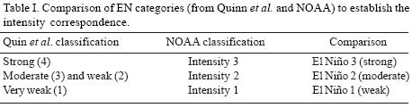
<body><![CDATA[<p align="justify"><font face="verdana" size="2">NAS alterations in the geostrophic wind in the North Atlantic Ocean and a possible increase in the flows of cold air over Greenland, the Canadian Archipelago and even the Mediterranean Sea; while the warm advective streams in northern Europe increase their temperatures and drop in western North America (van Loon and Rogers, 1978). Rogers and van Loon (1979) described mid and high latitude variations in the atmosphere&#150;ocean&#150;cryosphere system associated to the seesaw. Likewise, Meehl and van Loon (1979) found that the seesaw has tropical teleconnections with the trade winds, the position of the intertropical convergence zone (ITCZ) in Africa, the sea temperature and the Gulf Stream intensity.</font></p>     <p align="justify"><font face="verdana" size="2">Several authors have found some statistical relations between NAO and El Ni&ntilde;o (EN). For example, Rogers (1984) found that significant sea level pressure differences are correlated with these teleconnections over much of the Northern Hemisphere, even though for 80 winter years with data simultaneous appearance of both modes seemed to occur by chance <i>(e.g. </i>Hurrell <i>et al., </i>2001; Wanner <i>et al., </i>2001). According to Fraedrich (1994) noise level seemed to mask out atmospheric teleconnections.</font></p>     <p align="justify"><font face="verdana" size="2">The objective of this study is to estimate the probability of simultaneous occurrence between the four modalities of NAS and the three intensities of EN, during the winter months (in the Northern Hemisphere) along the period 1840&#150;1990. It is necessary to point out that, although both NAS and EN occur during the northern winter months (explained in the next section), EN can span over a longer period, even reaching up to two years in some cases. However, and with the purpose of establishing the link between both events, each one of them was considered as a phenomenon of winter months, according to van Loon and Rogers (1978).</font></p>     <p align="justify"><font face="verdana" size="2">&nbsp;</font></p>     <p align="justify"><font face="verdana" size="2"><b>2. Data and method</b></font></p>     <p align="justify"><font face="verdana" size="2">In order to establish the probability of simultaneous occurrence of NAS and EN, records of EN were gathered from the classification proposed by Quinn <i>et al. </i>(1978). The authors categorize EN events recorded during the period 1726&#150;1976, regarding the intensity of the event as much as its duration, in four categories: strong (4), moderate (3), weak (2), and very weak (1); based on nine indicators: 1) reports of perturbations on the anchovy fisheries and on the marine populations of birds of the Peruvian coasts; 2) scientific records reporting low phytoplankton production in the coastal regions of Per&uacute; and southern Ecuador; 3) hydrological data from the coast of Peru showing nutrient reduction; 4) records of sea surface temperature along the coasts of Peru and Southern Ecuador, where an alteration in the position of the thermocline was evidenced; 5) rainfall positive anomalies in the coastal stations of Per&uacute; and southern Ecuador; 6) alteration in the tendencies of the Southern Oscillation Index; 7) factors related to changes in the barometric pressure; 8) increment of sea surface temperature in the equatorial Pacific Ocean; and 9) anomalous negative rain records in the islands of the central and western equatorial Pacific Ocean.</font></p>     <p align="justify"><font face="verdana" size="2">In order to complete the studied period, EN records during 1977&#150;1990 were taken from NOAA (2004). On the other hand, Quinn <i>et al. </i>'s (1978) record was cut away from 1726 to 1839, to have the same period for both phenomena (EN and NAS). For the purposes of this work, EN files from both sources were compared and transformed into three categories (intensities) according to NOAA classification (<a href="#t1">Table I</a>).</font></p>     <p align="center"><font face="verdana" size="2"><a name="t1"></a></font></p>     <p align="center"><font face="verdana" size="2"><img src="/img/revistas/atm/v20n1/a3t1.jpg"></font></p>     <p align="justify"><font face="verdana" size="2">NAS records during the period 1840&#150;1990 were taken from the World Weather Records (1929, 1934, 1947, 1959, 1965, 1966, 1979a, 1979b, 1987, 1989, 1995, 1996) and classified according to van Loon and Rogers' (1978) characterization as follows. First, the average monthly temperature for November, December, January and February, considered in this paper as winter months according to Labitzke and van Loon (1988) and Rodr&iacute;guez&#150;Fonseca <i>et al. </i>(2004), was calculated for Greenland (Jacobshavn) and Norway (Oslo). From this mean, the temperature anomaly was determined, separating the anomalies whose absolute value exceeded from 1 &deg;C and have the same sign; and those having opposite signs with a difference of at least 1 &deg;C between both. In order to compare the temperature differences that define the homogeneous and heterogeneous modalities, we lowered the van Loon and Rogers' (1978) range of the heterogeneous ones from 4 to 1 &deg;C. Then, they were grouped in four modalities: BA, BB, GA and GB. Afterwards, the number of NAS occurred in every month was determined by a frequency chart for the period 1840&#150;1990.</font></p>     ]]></body>
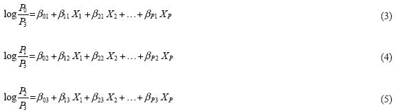
<body><![CDATA[<p align="justify"><font face="verdana" size="2">The data of EN and NAS were grouped in winters, so the same winter season consists in four months: November and December of one year, and January and February of the next one. Therefore, the 150 winter seasons of the 151 years were obtained, eliminating January and February 1840, and November and December 1990; so we have 600 winter months in total.</font></p>     <p align="justify"><font face="verdana" size="2">To determine whether the probability of NAS and EN occurrence is completely random or if the probability of EN occurrence is a function of NAS presence and modality, models of dichotomic (presence/absence) and polytomic (with more than two attributes for the dependent variable) logistic regressions were used. The fit of models was done with the program JMP, using robust variance estimates to account for clusters of months in each of the 150 winter seasons. The logistic models were analyzed according to Hosmer and Lemeshow (1989). In every case, EN intensities were considered as dependent while NAS modalities and the winter months were considered as independent.</font></p>     <p align="justify"><font face="verdana" size="2">The equation for the dichotomic logistic pattern is:</font></p>     <p align="justify"><font face="verdana" size="2">where <i>P<sub>i</sub> </i>is the probability of the event I (i = 1, 2), for example EN occurrence, and X<sub>i</sub>,. <i>X<sub>p</sub> </i>are the independent variables. Once the &beta; values are computed, probabilities for each category of dependent</font></p>     <p align="justify"><font face="verdana" size="2"><i><img src="/img/revistas/atm/v20n1/a3s1.jpg"></i></font></p>     <p align="justify"><font face="verdana" size="2">variables are estimated, according to Brant (1996) as:</font></p>     <p align="justify"><font face="verdana" size="2"><img src="/img/revistas/atm/v20n1/a3s2.jpg"></font></p>     <p align="justify"><font face="verdana" size="2"><i>X<sub>1</sub>... X<sub>p</sub> </i>are the values of the independent variables, with indicator variables for categorical independence.</font></p>     <p align="justify"><font face="verdana" size="2">The model equations for the polytomic logistic (multinomial with i = 0, 1, 2, 3) are:</font></p>     <p align="justify"><font face="verdana" size="2"><img src="/img/revistas/atm/v20n1/a3s3.jpg"></font></p>     ]]></body>
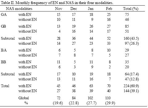
<body><![CDATA[<p align="justify"><font face="verdana" size="2">with the restriction <i>P<sub>0</sub> + P<sub>1</sub> + P<sub>2</sub> + P<sub>3</sub> = </i>1.</font></p>     <p align="justify"><font face="verdana" size="2">The values of &beta; coefficients are specific for each equation. <i>P<sub>0</sub> </i>is the probability of EN absent (i = 0), <i>P<sub>i</sub></i>, the probability of EN intensity i (i = 1, 2, 3).</font></p>     <p align="justify"><font face="verdana" size="2">When the values of the logistic &beta; regression coefficients are determined, the estimated probabilities for each NAS modalities are found, from the above four equations.</font></p>     <p align="justify"><font face="verdana" size="2">The goodness of fit of the predicted probabilities with the observed frequencies was computed through a &chi;<sup>2</sup> test, for &alpha; &lt; 0.05, where <i>H<sub>0</sub>: </i>there are no statistical differences between the observed frequencies and the predicted probabilities; versus <i>H<sub>a:</sub> </i>there are differences between observed and predicted. If <i>H<sub>0</sub> </i>is not rejected, then the model is acceptable.</font></p>     <p align="justify"><font face="verdana" size="2">&nbsp;</font></p>     <p align="justify"><font face="verdana" size="2"><b>3. Results</b></font></p>     <p align="justify"><font face="verdana" size="2">The statistical analyses were applied to EN and NAS records, covering the period 1840 to 1990, which amount to 151 years, 150 winter seasons and 600 winter months, as explained in the last section.</font></p>     <p align="justify"><font face="verdana" size="2">The results of the statistical analyses show that NAS frequency in its four modalities increases progressively as the northern winter advances, as it is shown in <a href="#t2">Table II</a>; 72 events are recorded in November, representing 19%; 84 in December (23%) ; 102 in January (28%); culminating with 110 (30%) in February.</font></p>     <p align="center"><font face="verdana" size="2"><a name="t2"></a></font></p>     <p align="center"><font face="verdana" size="2"><img src="/img/revistas/atm/v20n1/a3t2.jpg"></font></p>     ]]></body>
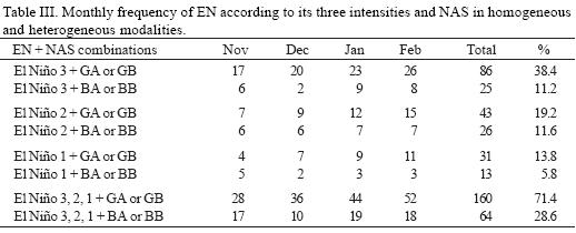
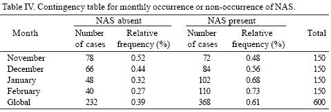
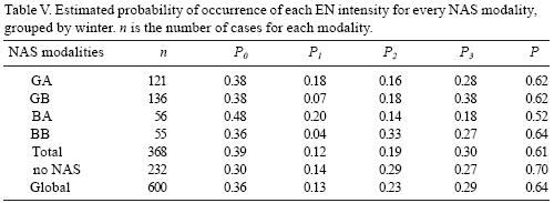
<body><![CDATA[<p align="justify"><font face="verdana" size="2">Regarding the simultaneity of occurrence of EN and NAS in their four modalities, from 368 cases of NAS observed, in 224 (60.9%) both events occurred; while in 144 cases (39.1%) only NAS occurred. These results imply that for NAS heterogeneous modalities coinciding with EN, 160 cases (43.5%) were recorded; while for homogeneous modalities, 64 cases (17.4%) occurred. The above implies that simultaneity of both events exists in 61% of the cases (<a href="#t2">Table II</a>).</font></p>     <p align="justify"><font face="verdana" size="2">Regarding EN intensities and NAS occurrence, a larger number of NAS events is recorded in their modalities GA or GB, when they coincide with intensity 3 (strong), which corresponds to 86 (38.4%). Occurrence decreases for those of intensity 2 (moderate) with 43 (19.2%) and finally for those of intensity 1 (weak) amounts 31 (13.8%). It is possible to affirm that from 224 observed cases, in 160 (71%) modalities GA or GB prevail; while 64 cases (29%) were recorded for modalities BA or BB (<a href="#t3">Table III</a>).</font></p>     <p align="center"><font face="verdana" size="2"><a name="t3"></a></font></p>     <p align="center"><font face="verdana" size="2"><img src="/img/revistas/atm/v20n1/a3t3.jpg"></font></p>     <p align="justify"><font face="verdana" size="2">In first instance, the probability of NAS occurrence was determined (dependent variable) in its homogeneous and heterogeneous modalities, expressed as yes/no in a contingency table during the northern winter months (independent variable) (<a href="#t4">Table IV</a>). The logistic model showed a<i> p = </i>0.0001, corrected by the correlations within winters. This table shows that the relative frequency of a NAS event occurring during the winter months is on the average of 61% <i>vs </i>an average of 39% that it does not occur. In addition, it stands out that as the winter months progress, there is an increase in NAS relative frequency, particularly in February (73%).</font></p>     <p align="center"><font face="verdana" size="2"><a name="t4"></a></font></p>     <p align="center"><font face="verdana" size="2"><img src="/img/revistas/atm/v20n1/a3t4.jpg"></font></p>     <p align="justify"><font face="verdana" size="2">Next, the probability of occurrence of EN was estimated with a logistic model adjusted by winter, considering EN as dependent and NAS as independent, and categorizing NAS only as present&#150;absent. In the model the four northern winter months were included, however, when considering NAS incidence per month, the interaction was not significant; therefore this model was discarded and another was proposed where only the main effects of month and NAS were included, that is to say, the probability of EN occurrence as a function of NAS and of the month. In this model a &chi;<sup>2</sup> = 27.57 is obtained with three degrees of freedom and p = 0.0001, which leads to the rejection of the hypothesis of independence.</font></p>     <p align="justify"><font face="verdana" size="2">Regarding the main effects in the model, only NAS was significant <i>(p <u>&lt;</u> </i>0.03 in likelihood ratio test), and for month p was 0.91. The probabilities of EN occurrence according to NAS modalities adjusted by month are of 0.70 if there is no NAS and of 0.61 when NAS occurs (<a href="#t5">Table V</a>).</font></p>     <p align="center"><font face="verdana" size="2"><a name="t5"></a></font></p>     ]]></body>
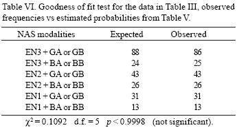
<body><![CDATA[<p align="center"><font face="verdana" size="2"><img src="/img/revistas/atm/v20n1/a3t5.jpg"></font></p>     <p align="justify"><font face="verdana" size="2">Then, a new model of logistic regression was used, where EN presence/absence was considered as dependent variable, and the month and NAS with four modalities as independent. The interaction effect between type and month was not significant. Even though none of the main effects was significant, one of the indicator variables for NAS was significant with p &lt; 0.013 in Wald test. With this model, the estimated probabilities <i>(P) </i>of EN occurrence were obtained for each NAS modality, corrected per month (last column of <a href="#t5">Table V</a>), BB, GB and GA stand out in order of magnitude, with the lowest probability of EN occurrence of 0.52 with NAS modality BA.</font></p>     <p align="justify"><font face="verdana" size="2">A last model of polytomic logistic regression was used to estimate the probability <i>P<sub>i</sub></i> of occurrence of each EN intensity (i), with its four intensities as dependent variable, and with the month and NAS modalities as independent, grouped for every winter; it was found that there was no significant interaction. While this model was not significant for month <i>(p &lt; </i>0.51), it was highly significant for NAS modality <i>(p &lt; </i>0.0004). With this model, probabilities adjusted per month were obtained for each EN intensity <i>(P<i><sub>i</sub></i>, P<sub>0</sub> </i>means absence of EN) and for each NAS modality (<a href="#t5">Table V</a>).</font></p>     <p align="justify"><font face="verdana" size="2">The higher probabilities of occurrence of an EN intensity 3 event in the heterogeneous modalities of NAS stand out, amounting to 0.66 as a whole, which confirms the results obtained by the frequency chart (<a href="#t3">Table III</a>); while, in NAS homogeneous modalities with EN intensity 3, they amount to 0.45 as a whole. The lowest intensity of EN had the low probability of 0.04 with BB NAS, and the highest intensity is more probable with the other modalities of NAS, reaching 0.38 with GB.</font></p>     <p align="justify"><font face="verdana" size="2">In order to determine the goodness of fit of the frequencies predicted by the polytomic model and the observed ones, a &chi;<sup>2</sup> test was performed for the different NAS modalities, considering each winter season as a whole. These results are presented in <a href="#t6">Table VI</a>.</font></p>     <p align="center"><font face="verdana" size="2"><a name="t6"></a></font></p>     <p align="center"><font face="verdana" size="2"><img src="/img/revistas/atm/v20n1/a3t6.jpg"></font></p>     <p align="justify"><font face="verdana" size="2">Thus, <i>H<sub>0</sub> </i>is not rejected, and the <i>p </i>value proves that there is a very close fit of the observed data to the probabilities predicted by the model, at least for the whole winter season.</font></p>     <p align="justify"><font face="verdana" size="2">&nbsp;</font></p>     <p align="justify"><font face="verdana" size="2"><b>4. Discussion</b></font></p>     ]]></body>
<body><![CDATA[<p align="justify"><font face="verdana" size="2">Although the present paper is basically probabilistic, some other correlations and physical mechanisms support our statement that the results of the model are not spurious, but are instead based on the link between both phenomena.</font></p>     <p align="justify"><font face="verdana" size="2">Van Loon and Rogers (1978) explain some processes at the northern mid and high latitudes related to the seesaw. Rogers and van Loon (1979) described the variations in atmosphere, ocean and cryosphere associated to the seesaw at those same latitudes. Meehl and van Loon (1979) find that the seesaw has tropical teleconnections, other than EN.</font></p>     <p align="justify"><font face="verdana" size="2">Many studies about the relations and teleconnections between atmosphere and ocean have been carried out, over a wide span of time and with a global scope. Some of the most classic and important are those of Bjerknes (1964, 1965, 1966, 1969). Nevertheless, an alternative hypothesis is that there is a coupling between tropospheric and stratospheric circulations; some researchers have found statistical correlations between the strength of the stratospheric winter vortex and the tropospheric circulation over the North Atlantic (Perlwitz and Graf, 1995; Kodera <i>et al., </i>1996; 1999), supported with the results by Wanner <i>et al. </i>(2001), who found significant correlations between geopotential height over the North Atlantic and the wintertime Index of NAO (NAOI), which were even higher for the Index of Artic Oscillation (AOI), up to the 5 0 hPa levels, thus revealing that the NAO/AO signal encompasses the whole troposphere and lower stratosphere of this region.</font></p>     <p align="justify"><font face="verdana" size="2">Even though the mechanisms are not well understood, some authors have found a coupling between the conditions at the tropical Pacific Ocean and those at the North Atlantic <i>(e.g. </i>Bjerknes, 1966). There are models predicting that the development of permanent El Ni&ntilde;o conditions would increase freshwater flow from the Atlantic into other basins (Timmermann <i>et al., </i>1999; Latif <i>et al. </i>2000) and thus that the interaction involves the ocean as well as the atmosphere. On the other hand, Rogers (1984) found that, over most of the Northern Hemisphere, both ENSO and NAO associate to significant sea level pressure differences.</font></p>     <p align="justify"><font face="verdana" size="2">One important aspect of the present work is the proposal of the probabilistic estimation method by using polytomic logistic models, which are statistical tools with little use in climatic studies. The validity of this method is further increased when the record of events is quantitative, as NAS and EN, whose categorization was implemented since the late 1970s. This feature facilitates the statistical analysis in series longer than 100 years, with a confidence level higher than 95%. Other important aspect is that the analysis was performed from a series that includes more years than the series used by other researchers (1840&#150;1990). Both of these facts resulted in a close fit between the observed data and the model results, at least for the probabilities for the whole winter season.</font></p>     <p align="justify"><font face="verdana" size="2">Nevertheless, a close look at <a href="#t5">Table V</a> shows that, for heterogeneous modalities, the probability of having a strong EN or not having EN is almost the same (0.28 to 0.38), a fact that limits its practical applicability for prediction, at least while further causes are not found that would define the most likely outcome for a particular season. On the other hand, for BA homogeneous modality the probability of not having EN is close to 50%.</font></p>     <p align="justify"><font face="verdana" size="2">&nbsp;</font></p>     <p align="justify"><font face="verdana" size="2"><b>5. Conclusions</b></font></p>     <p align="justify"><font face="verdana" size="2">This analysis was performed using long series of historical records (one and a half centuries, or 600 winter months) for NAS and EN, which renders a probabilistic strength.The incidence of NAS events increases as the northern winter advances.</font></p>     <blockquote>       ]]></body>
<body><![CDATA[<p align="justify"><font face="verdana" size="2">NAS heterogeneous modalities (GA and GB) coincide in 71 % with EN events, while homogeneous modalities (BA and BB) do so in 29%.</font></p>       <p align="justify"><font face="verdana" size="2">NAS heterogeneous modalities (GA and GB) for EN occurrence have a higher coincidence with EN intensity 3.</font></p>       <p align="justify"><font face="verdana" size="2">The simultaneity of the NAS and EN occurs in 61% of cases.</font></p>       <p align="justify"><font face="verdana" size="2">For heterogeneous NAS modalities, the expected relative frequency of having EN is close to 50%.</font></p>       <p align="justify"><font face="verdana" size="2">There is a close fit between the probabilities predicted by the logistic polytomic model and the observed frequencies.</font></p>       <p align="justify"><font face="verdana" size="2">There is a close fit between the observed frequencies and the model predicted probability for the NAS modalities, at least for the whole winter season.</font></p> </blockquote>     <p align="justify"><font face="verdana" size="2">&nbsp;</font></p>     <p align="justify"><font face="verdana" size="2"><b>Acknowledgment</b></font></p>     <p align="justify"><font face="verdana" size="2">Comments on the original manuscript by two anonymous reviewers are greatly appreciated.</font></p>     <p align="justify"><font face="verdana" size="2">&nbsp;</font></p>     ]]></body>
<body><![CDATA[<p align="justify"><font face="verdana" size="2"><b>References</b></font></p>     <!-- ref --><p align="justify"><font face="verdana" size="2">Bjerknes J., 1964. Atlantic air&#150;sea interaction. <i>Adv. Geophys. </i><b>10</b>, 1&#150;82.</font>&nbsp;&nbsp;&nbsp;&nbsp;&nbsp;&nbsp;&nbsp;&nbsp;[&#160;<a href="javascript:void(0);" onclick="javascript: window.open('/scielo.php?script=sci_nlinks&ref=1268198&pid=S0187-6236200700010000300001&lng=','','width=640,height=500,resizable=yes,scrollbars=1,menubar=yes,');">Links</a>&#160;]<!-- end-ref --><!-- ref --><p align="justify"><font face="verdana" size="2">Bjerknes J., 1965. Atmosphere&#150;ocean interaction during the '<sup>'</sup>Little Ice Age<sup>'</sup>' (seventeenth to nineteenth centuries, AD). In: World Meteorological Organization&#150;IUGG. Symposium on Research and Development Aspects of Longe&#150;Range Forecasting. Technical Note 66. WMO&#150;No. 162. TP. 79, 77&#150;88.</font>&nbsp;&nbsp;&nbsp;&nbsp;&nbsp;&nbsp;&nbsp;&nbsp;[&#160;<a href="javascript:void(0);" onclick="javascript: window.open('/scielo.php?script=sci_nlinks&ref=1268199&pid=S0187-6236200700010000300002&lng=','','width=640,height=500,resizable=yes,scrollbars=1,menubar=yes,');">Links</a>&#160;]<!-- end-ref --><!-- ref --><p align="justify"><font face="verdana" size="2">Bjerknes J., 1966. A possible response of the atmospheric Hadley circulation to equatorial anomalies of ocean temperature. <i>Tellus </i><b>18</b>, 820&#150;829.</font>&nbsp;&nbsp;&nbsp;&nbsp;&nbsp;&nbsp;&nbsp;&nbsp;[&#160;<a href="javascript:void(0);" onclick="javascript: window.open('/scielo.php?script=sci_nlinks&ref=1268200&pid=S0187-6236200700010000300003&lng=','','width=640,height=500,resizable=yes,scrollbars=1,menubar=yes,');">Links</a>&#160;]<!-- end-ref --><!-- ref --><p align="justify"><font face="verdana" size="2">Bjerknes J., 1969. Atmospheric teleconnections from the equatorial Pacific. Mon. <i>Wea. Rev., </i><b>97</b>, 163&#150;172.    &nbsp;&nbsp;&nbsp;&nbsp;&nbsp;&nbsp;&nbsp;&nbsp;[&#160;<a href="javascript:void(0);" onclick="javascript: window.open('/scielo.php?script=sci_nlinks&ref=1268201&pid=S0187-6236200700010000300004&lng=','','width=640,height=500,resizable=yes,scrollbars=1,menubar=yes,');">Links</a>&#160;]<!-- end-ref --><!-- ref --> Brant R., 1996. Digesting logistic regression results. <i>Am. Stat. </i><b>50</b>, 117&#150;119.</font>&nbsp;&nbsp;&nbsp;&nbsp;&nbsp;&nbsp;&nbsp;&nbsp;[&#160;<a href="javascript:void(0);" onclick="javascript: window.open('/scielo.php?script=sci_nlinks&ref=1268202&pid=S0187-6236200700010000300005&lng=','','width=640,height=500,resizable=yes,scrollbars=1,menubar=yes,');">Links</a>&#160;]<!-- end-ref --><!-- ref --><p align="justify"><font face="verdana" size="2">Dawson A. G., L. Elliott, P. Mayewski, P. Lockett, S. Noone, K. Hickey, T. Holt, P. Wadhams and I. D. L. Foster, 2003. Late&#150;Holocene North Atlantic climate '<sup>'</sup>seesaws<sup>'</sup>', storminess changes and Greenland ice sheet (GISP2) palaeoclimates. <i>Holocene </i><b>13</b>, 381&#150;392.</font>&nbsp;&nbsp;&nbsp;&nbsp;&nbsp;&nbsp;&nbsp;&nbsp;[&#160;<a href="javascript:void(0);" onclick="javascript: window.open('/scielo.php?script=sci_nlinks&ref=1268203&pid=S0187-6236200700010000300006&lng=','','width=640,height=500,resizable=yes,scrollbars=1,menubar=yes,');">Links</a>&#160;]<!-- end-ref --><!-- ref --><p align="justify"><font face="verdana" size="2">Fraedrich K., 1994. An ENSO impact on Europe? A review. <i>Tellus </i><b>46A</b>, 541&#150;552.</font>&nbsp;&nbsp;&nbsp;&nbsp;&nbsp;&nbsp;&nbsp;&nbsp;[&#160;<a href="javascript:void(0);" onclick="javascript: window.open('/scielo.php?script=sci_nlinks&ref=1268204&pid=S0187-6236200700010000300007&lng=','','width=640,height=500,resizable=yes,scrollbars=1,menubar=yes,');">Links</a>&#160;]<!-- end-ref --><!-- ref --><p align="justify"><font face="verdana" size="2">Greatbatch R. J., 2000. The North Atlantic Oscillation. <i>Stoch. Env. Res. Risk Assess. </i><b>14</b>, 213&#150;242.</font>&nbsp;&nbsp;&nbsp;&nbsp;&nbsp;&nbsp;&nbsp;&nbsp;[&#160;<a href="javascript:void(0);" onclick="javascript: window.open('/scielo.php?script=sci_nlinks&ref=1268205&pid=S0187-6236200700010000300008&lng=','','width=640,height=500,resizable=yes,scrollbars=1,menubar=yes,');">Links</a>&#160;]<!-- end-ref --><!-- ref --><p align="justify"><font face="verdana" size="2">Hosmer D. W. and S. Lemeshow, 1989. <i>Applied logistic regression. </i>John Wiley and Sons. New York, 307 p.</font>&nbsp;&nbsp;&nbsp;&nbsp;&nbsp;&nbsp;&nbsp;&nbsp;[&#160;<a href="javascript:void(0);" onclick="javascript: window.open('/scielo.php?script=sci_nlinks&ref=1268206&pid=S0187-6236200700010000300009&lng=','','width=640,height=500,resizable=yes,scrollbars=1,menubar=yes,');">Links</a>&#160;]<!-- end-ref --><!-- ref --><p align="justify"><font face="verdana" size="2">Hurrell J. W., 1996. Influence of variations in extratropical wintertime teleconnections on Northern Hemisphere temperature. <i>Geophys. Res. Lett. </i><b>23</b>, 665&#150;668.</font>&nbsp;&nbsp;&nbsp;&nbsp;&nbsp;&nbsp;&nbsp;&nbsp;[&#160;<a href="javascript:void(0);" onclick="javascript: window.open('/scielo.php?script=sci_nlinks&ref=1268207&pid=S0187-6236200700010000300010&lng=','','width=640,height=500,resizable=yes,scrollbars=1,menubar=yes,');">Links</a>&#160;]<!-- end-ref --><!-- ref --><p align="justify"><font face="verdana" size="2">Hurrell J. W., Y. Kushnir and M. Visbeck, 2001. The North Atlantic Oscillation. <i>Science, </i><b>291</b>, 603&#150;605.</font>&nbsp;&nbsp;&nbsp;&nbsp;&nbsp;&nbsp;&nbsp;&nbsp;[&#160;<a href="javascript:void(0);" onclick="javascript: window.open('/scielo.php?script=sci_nlinks&ref=1268208&pid=S0187-6236200700010000300011&lng=','','width=640,height=500,resizable=yes,scrollbars=1,menubar=yes,');">Links</a>&#160;]<!-- end-ref --><!-- ref --><p align="justify"><font face="verdana" size="2">Kodera K., M. Chiba, H. Koide, A. Kitoh and Y. Nikaidou, 1996. Interannual variability of the winter stratosphere and troposphere in the Northern Hemisphere. <i>J. Meteor. Soc. Japan </i><b>74</b>, 365&#150;382.</font>&nbsp;&nbsp;&nbsp;&nbsp;&nbsp;&nbsp;&nbsp;&nbsp;[&#160;<a href="javascript:void(0);" onclick="javascript: window.open('/scielo.php?script=sci_nlinks&ref=1268209&pid=S0187-6236200700010000300012&lng=','','width=640,height=500,resizable=yes,scrollbars=1,menubar=yes,');">Links</a>&#160;]<!-- end-ref --><!-- ref --><p align="justify"><font face="verdana" size="2">Kodera K., H. Koide and H. Yoshimura, 1999. Northern Hemisphere winter circulation associated with the North Atlantic Oscillation and stratospheric polar&#150;night jet. <i>Geophys. Res. Lett. </i><b>26</b>, 443&#150;446.</font>&nbsp;&nbsp;&nbsp;&nbsp;&nbsp;&nbsp;&nbsp;&nbsp;[&#160;<a href="javascript:void(0);" onclick="javascript: window.open('/scielo.php?script=sci_nlinks&ref=1268210&pid=S0187-6236200700010000300013&lng=','','width=640,height=500,resizable=yes,scrollbars=1,menubar=yes,');">Links</a>&#160;]<!-- end-ref --><!-- ref --><p align="justify"><font face="verdana" size="2">Labitzke K. and H. van Loon, 1988. Association between the 11&#150;year solar cycle, the QBO and the atmosphere. Part I: The troposphere and stratosphere in the Northern Hemisphere in winter. <i>J. Atmos. Terr. Phys. </i><b>50</b>, 197&#150;206.</font>&nbsp;&nbsp;&nbsp;&nbsp;&nbsp;&nbsp;&nbsp;&nbsp;[&#160;<a href="javascript:void(0);" onclick="javascript: window.open('/scielo.php?script=sci_nlinks&ref=1268211&pid=S0187-6236200700010000300014&lng=','','width=640,height=500,resizable=yes,scrollbars=1,menubar=yes,');">Links</a>&#160;]<!-- end-ref --><!-- ref --><p align="justify"><font face="verdana" size="2">Latif M., K. Arpe and E. Roeckner, 2000. Oceanic control of decadal North Atlantic sea level pressure variability in winter. <i>Geophys. Res. Lett. </i><b>27</b>, 727&#150;730.</font>&nbsp;&nbsp;&nbsp;&nbsp;&nbsp;&nbsp;&nbsp;&nbsp;[&#160;<a href="javascript:void(0);" onclick="javascript: window.open('/scielo.php?script=sci_nlinks&ref=1268212&pid=S0187-6236200700010000300015&lng=','','width=640,height=500,resizable=yes,scrollbars=1,menubar=yes,');">Links</a>&#160;]<!-- end-ref --><!-- ref --><p align="justify"><font face="verdana" size="2">Loewe F., 1937. A period of warm winters in western Greenland and the temperature seesaw between western Greenland and central Europe. <i>Quart. J. Roy. Meteor. Soc. </i><b>63</b>, 365&#150;372.</font>&nbsp;&nbsp;&nbsp;&nbsp;&nbsp;&nbsp;&nbsp;&nbsp;[&#160;<a href="javascript:void(0);" onclick="javascript: window.open('/scielo.php?script=sci_nlinks&ref=1268213&pid=S0187-6236200700010000300016&lng=','','width=640,height=500,resizable=yes,scrollbars=1,menubar=yes,');">Links</a>&#160;]<!-- end-ref --><!-- ref --><p align="justify"><font face="verdana" size="2">Loewe F., 1966. The temperature seesaw between western Greenland and Europe. <i>Weather </i><b>21</b>, 241&#150;246.</font>&nbsp;&nbsp;&nbsp;&nbsp;&nbsp;&nbsp;&nbsp;&nbsp;[&#160;<a href="javascript:void(0);" onclick="javascript: window.open('/scielo.php?script=sci_nlinks&ref=1268214&pid=S0187-6236200700010000300017&lng=','','width=640,height=500,resizable=yes,scrollbars=1,menubar=yes,');">Links</a>&#160;]<!-- end-ref --><!-- ref --><p align="justify"><font face="verdana" size="2">Meehl G. A. and H. van Loon, 1979. The seesaw in winter temperatures between Greenland and northern Europe. Part III: Teleconnections with lower latitudes. <i>Mon. Wea. Rev. </i><b>107</b>, 1095&#150;1106.</font>&nbsp;&nbsp;&nbsp;&nbsp;&nbsp;&nbsp;&nbsp;&nbsp;[&#160;<a href="javascript:void(0);" onclick="javascript: window.open('/scielo.php?script=sci_nlinks&ref=1268215&pid=S0187-6236200700010000300018&lng=','','width=640,height=500,resizable=yes,scrollbars=1,menubar=yes,');">Links</a>&#160;]<!-- end-ref --><!-- ref --><p align="justify"><font face="verdana" size="2">NOAA, 2004. <A href=http://www.cpc.ncep.noaa.gov/data/indices target="_blank">http://www.cpc.ncep.noaa.gov/data/indices</A>.</font>&nbsp;&nbsp;&nbsp;&nbsp;&nbsp;&nbsp;&nbsp;&nbsp;[&#160;<a href="javascript:void(0);" onclick="javascript: window.open('/scielo.php?script=sci_nlinks&ref=1268216&pid=S0187-6236200700010000300019&lng=','','width=640,height=500,resizable=yes,scrollbars=1,menubar=yes,');">Links</a>&#160;]<!-- end-ref --><!-- ref --><p align="justify"><font face="verdana" size="2">Perlwitz J. and H.&#150;F. Graf, 1995. The statistical connection between tropospheric and stratospheric circulation of the Northern Hemisphere in winter. <i>J. Climate </i><b>8</b>, 2281&#150;2295.</font>&nbsp;&nbsp;&nbsp;&nbsp;&nbsp;&nbsp;&nbsp;&nbsp;[&#160;<a href="javascript:void(0);" onclick="javascript: window.open('/scielo.php?script=sci_nlinks&ref=1268217&pid=S0187-6236200700010000300020&lng=','','width=640,height=500,resizable=yes,scrollbars=1,menubar=yes,');">Links</a>&#160;]<!-- end-ref --><!-- ref --><p align="justify"><font face="verdana" size="2">Quinn W. H., D. O. Zopf, K. S. Short and R. T. W. Kuo Yang, 1978. Historical trends and statistics of the Southern Oscillation, El Ni&ntilde;o, and Indonesian droughts. <i>Fish. Bull. </i><b>76</b>, 663&#150;678.</font>&nbsp;&nbsp;&nbsp;&nbsp;&nbsp;&nbsp;&nbsp;&nbsp;[&#160;<a href="javascript:void(0);" onclick="javascript: window.open('/scielo.php?script=sci_nlinks&ref=1268218&pid=S0187-6236200700010000300021&lng=','','width=640,height=500,resizable=yes,scrollbars=1,menubar=yes,');">Links</a>&#160;]<!-- end-ref --><!-- ref --><p align="justify"><font face="verdana" size="2">Rodr&iacute;guez&#150;Fonseca B., I. Polo, E. Serrano and M. de Castro, 2004. A subtropical Atlantic predictor of winter anomalous precipitation in the Iberian peninsula, some European regions and the north of Africa. <i>Int. J. Climatol. </i>(accepted).</font>&nbsp;&nbsp;&nbsp;&nbsp;&nbsp;&nbsp;&nbsp;&nbsp;[&#160;<a href="javascript:void(0);" onclick="javascript: window.open('/scielo.php?script=sci_nlinks&ref=1268219&pid=S0187-6236200700010000300022&lng=','','width=640,height=500,resizable=yes,scrollbars=1,menubar=yes,');">Links</a>&#160;]<!-- end-ref --><!-- ref --><p align="justify"><font face="verdana" size="2">Rogers J. C., 1984. The association between the North Atlantic Oscillation and the Southern Oscillation in the Northern Hemisphere. <i>Mon. Wea. Rev. </i><b>112</b>, 1999&#150;2015.</font>&nbsp;&nbsp;&nbsp;&nbsp;&nbsp;&nbsp;&nbsp;&nbsp;[&#160;<a href="javascript:void(0);" onclick="javascript: window.open('/scielo.php?script=sci_nlinks&ref=1268220&pid=S0187-6236200700010000300023&lng=','','width=640,height=500,resizable=yes,scrollbars=1,menubar=yes,');">Links</a>&#160;]<!-- end-ref --><!-- ref --><p align="justify"><font face="verdana" size="2">Rogers J. C., and H. van Loon, 1979. The seesaw in winter temperatures between Greenland and northern Europe. Part II: Some oceanic and atmospheric effects in middle and high latitudes. <i>Mon. Wea. Rev. </i><b>107</b>, 509&#150;519.</font>&nbsp;&nbsp;&nbsp;&nbsp;&nbsp;&nbsp;&nbsp;&nbsp;[&#160;<a href="javascript:void(0);" onclick="javascript: window.open('/scielo.php?script=sci_nlinks&ref=1268221&pid=S0187-6236200700010000300024&lng=','','width=640,height=500,resizable=yes,scrollbars=1,menubar=yes,');">Links</a>&#160;]<!-- end-ref --><!-- ref --><p align="justify"><font face="verdana" size="2">Timmermann A., J. Oberhuber, A. Bacher, M. Esch, M. Latif, and E. Roeckner, 1999. Increased El Ni&ntilde;o frequency in a climate model forced by future greenhouse warming. <i>Nature </i><b>398</b>, 694&#150;696.</font>&nbsp;&nbsp;&nbsp;&nbsp;&nbsp;&nbsp;&nbsp;&nbsp;[&#160;<a href="javascript:void(0);" onclick="javascript: window.open('/scielo.php?script=sci_nlinks&ref=1268222&pid=S0187-6236200700010000300025&lng=','','width=640,height=500,resizable=yes,scrollbars=1,menubar=yes,');">Links</a>&#160;]<!-- end-ref --><!-- ref --><p align="justify"><font face="verdana" size="2">Van Loon H. and J. C. Rogers, 1978. The seesaw in winter temperatures between Greenland and northern Europe. Part I: General description. <i>Mon. Wea. Rev. </i><b>106</b>, 296&#150;310.</font>&nbsp;&nbsp;&nbsp;&nbsp;&nbsp;&nbsp;&nbsp;&nbsp;[&#160;<a href="javascript:void(0);" onclick="javascript: window.open('/scielo.php?script=sci_nlinks&ref=1268223&pid=S0187-6236200700010000300026&lng=','','width=640,height=500,resizable=yes,scrollbars=1,menubar=yes,');">Links</a>&#160;]<!-- end-ref --><!-- ref --><p align="justify"><font face="verdana" size="2">Wanner H., S. Br&ouml;nnimann, C. Casty, D. Gyalistras, J. Luterbacher, C. Schmutz, D. B. Stephenson and E. Xoplaki, 2001. North Atlantic Oscillation &#150; concepts and studies. <i>Surv. Geophys. </i><b>22</b>, 321&#150;382.</font>&nbsp;&nbsp;&nbsp;&nbsp;&nbsp;&nbsp;&nbsp;&nbsp;[&#160;<a href="javascript:void(0);" onclick="javascript: window.open('/scielo.php?script=sci_nlinks&ref=1268224&pid=S0187-6236200700010000300027&lng=','','width=640,height=500,resizable=yes,scrollbars=1,menubar=yes,');">Links</a>&#160;]<!-- end-ref --><!-- ref --><p align="justify"><font face="verdana" size="2">World Weather Records, 1929. Volume 79. Smithsonian Miscellaneous Collections. Washington, D.C., 1199 p. </font>&nbsp;&nbsp;&nbsp;&nbsp;&nbsp;&nbsp;&nbsp;&nbsp;[&#160;<a href="javascript:void(0);" onclick="javascript: window.open('/scielo.php?script=sci_nlinks&ref=1268225&pid=S0187-6236200700010000300028&lng=','','width=640,height=500,resizable=yes,scrollbars=1,menubar=yes,');">Links</a>&#160;]<!-- end-ref --><!-- ref --><p align="justify"><font face="verdana" size="2">World Weather Records, 1934. <i>Continued from volume 79 1921&#150;1930. </i>Smithsonian Miscellaneous Collections. Washington, D.C. Vol. 90, Parts I and II, 616 p. </font>&nbsp;&nbsp;&nbsp;&nbsp;&nbsp;&nbsp;&nbsp;&nbsp;[&#160;<a href="javascript:void(0);" onclick="javascript: window.open('/scielo.php?script=sci_nlinks&ref=1268226&pid=S0187-6236200700010000300029&lng=','','width=640,height=500,resizable=yes,scrollbars=1,menubar=yes,');">Links</a>&#160;]<!-- end-ref --><!-- ref --><p align="justify"><font face="verdana" size="2">World Weather Records, 1947.<i>1931&#150;1940 (Continued from volumes 79 and 90) </i>Smithsonian Miscellaneous Collections. Washington, D.C. Vol. 105, Parts I and II, 646 p.</font>&nbsp;&nbsp;&nbsp;&nbsp;&nbsp;&nbsp;&nbsp;&nbsp;[&#160;<a href="javascript:void(0);" onclick="javascript: window.open('/scielo.php?script=sci_nlinks&ref=1268227&pid=S0187-6236200700010000300030&lng=','','width=640,height=500,resizable=yes,scrollbars=1,menubar=yes,');">Links</a>&#160;]<!-- end-ref --><!-- ref --><p align="justify"><font face="verdana" size="2">World Weather Records, 1959.<i>1941&#150;50. </i>U.S. Department of Commerce, Weather Bureau. Washington, D.C., 1361 p.</font>&nbsp;&nbsp;&nbsp;&nbsp;&nbsp;&nbsp;&nbsp;&nbsp;[&#160;<a href="javascript:void(0);" onclick="javascript: window.open('/scielo.php?script=sci_nlinks&ref=1268228&pid=S0187-6236200700010000300031&lng=','','width=640,height=500,resizable=yes,scrollbars=1,menubar=yes,');">Links</a>&#160;]<!-- end-ref --><!-- ref --><p align="justify"><font face="verdana" size="2"> World Weather Records, 1965.<i>1951&#150;60 Volume 1 North America. </i>U.S. Department of Commerce, Weather Bureau. Washington, D.C., 536 p. </font>&nbsp;&nbsp;&nbsp;&nbsp;&nbsp;&nbsp;&nbsp;&nbsp;[&#160;<a href="javascript:void(0);" onclick="javascript: window.open('/scielo.php?script=sci_nlinks&ref=1268229&pid=S0187-6236200700010000300032&lng=','','width=640,height=500,resizable=yes,scrollbars=1,menubar=yes,');">Links</a>&#160;]<!-- end-ref --><!-- ref --><p align="justify"><font face="verdana" size="2">World Weather Records, 1966.<i>1951&#150;60 Volume 2 Europe. </i>U.S. Department of Commerce, Environmental Science Services Administration. Washington, D.C., 548 p. </font>&nbsp;&nbsp;&nbsp;&nbsp;&nbsp;&nbsp;&nbsp;&nbsp;[&#160;<a href="javascript:void(0);" onclick="javascript: window.open('/scielo.php?script=sci_nlinks&ref=1268230&pid=S0187-6236200700010000300033&lng=','','width=640,height=500,resizable=yes,scrollbars=1,menubar=yes,');">Links</a>&#160;]<!-- end-ref --><!-- ref --><p align="justify"><font face="verdana" size="2">World Weather Records, 1979.<i>1961&#150;1970 Volume 1 North America. </i>U.S. Department of Commerce, NOAA. Asheville, N.C., 290 p. </font>&nbsp;&nbsp;&nbsp;&nbsp;&nbsp;&nbsp;&nbsp;&nbsp;[&#160;<a href="javascript:void(0);" onclick="javascript: window.open('/scielo.php?script=sci_nlinks&ref=1268231&pid=S0187-6236200700010000300034&lng=','','width=640,height=500,resizable=yes,scrollbars=1,menubar=yes,');">Links</a>&#160;]<!-- end-ref --><!-- ref --><p align="justify"><font face="verdana" size="2">World Weather Records, 1979.<i>1961&#150;1970 Volume 2 Europe. </i>U.S. Department of Commerce, NOAA. Asheville, N.C., 488 p.</font>&nbsp;&nbsp;&nbsp;&nbsp;&nbsp;&nbsp;&nbsp;&nbsp;[&#160;<a href="javascript:void(0);" onclick="javascript: window.open('/scielo.php?script=sci_nlinks&ref=1268232&pid=S0187-6236200700010000300035&lng=','','width=640,height=500,resizable=yes,scrollbars=1,menubar=yes,');">Links</a>&#160;]<!-- end-ref --><!-- ref --><p align="justify"><font face="verdana" size="2">World Weather Records, 1987.<i>1971 &#150;80 Volume 2 Europe. </i>U.S. Department of Commerce, NOAA, 399 p. </font>&nbsp;&nbsp;&nbsp;&nbsp;&nbsp;&nbsp;&nbsp;&nbsp;[&#160;<a href="javascript:void(0);" onclick="javascript: window.open('/scielo.php?script=sci_nlinks&ref=1268233&pid=S0187-6236200700010000300036&lng=','','width=640,height=500,resizable=yes,scrollbars=1,menubar=yes,');">Links</a>&#160;]<!-- end-ref --><!-- ref --><p align="justify"><font face="verdana" size="2">World Weather Records, 1989.<i>1971&#150;80 Volume 1 North America. </i>U.S. Department of Commerce, NOAA, 321 p. </font>&nbsp;&nbsp;&nbsp;&nbsp;&nbsp;&nbsp;&nbsp;&nbsp;[&#160;<a href="javascript:void(0);" onclick="javascript: window.open('/scielo.php?script=sci_nlinks&ref=1268234&pid=S0187-6236200700010000300037&lng=','','width=640,height=500,resizable=yes,scrollbars=1,menubar=yes,');">Links</a>&#160;]<!-- end-ref --><!-- ref --><p align="justify"><font face="verdana" size="2">World Weather Records, 1995.<i>1981&#150;90 Volume 2 Europe. </i>U.S. Department of Commerce, NOAA, 407 p. </font>&nbsp;&nbsp;&nbsp;&nbsp;&nbsp;&nbsp;&nbsp;&nbsp;[&#160;<a href="javascript:void(0);" onclick="javascript: window.open('/scielo.php?script=sci_nlinks&ref=1268235&pid=S0187-6236200700010000300038&lng=','','width=640,height=500,resizable=yes,scrollbars=1,menubar=yes,');">Links</a>&#160;]<!-- end-ref --><!-- ref --><p align="justify"><font face="verdana" size="2">World Weather Records, 1996.<i>1981&#150;90 Volume 1 North America. </i>U.S. Department of Commerce, NOAA, 313 p.</font>&nbsp;&nbsp;&nbsp;&nbsp;&nbsp;&nbsp;&nbsp;&nbsp;[&#160;<a href="javascript:void(0);" onclick="javascript: window.open('/scielo.php?script=sci_nlinks&ref=1268236&pid=S0187-6236200700010000300039&lng=','','width=640,height=500,resizable=yes,scrollbars=1,menubar=yes,');">Links</a>&#160;]<!-- end-ref --> ]]></body><back>
<ref-list>
<ref id="B1">
<nlm-citation citation-type="journal">
<person-group person-group-type="author">
<name>
<surname><![CDATA[Bjerknes]]></surname>
<given-names><![CDATA[J.]]></given-names>
</name>
</person-group>
<article-title xml:lang="en"><![CDATA[Atlantic air-sea interaction]]></article-title>
<source><![CDATA[Adv. Geophys.]]></source>
<year>1964</year>
<numero>10</numero>
<issue>10</issue>
<page-range>1-82</page-range></nlm-citation>
</ref>
<ref id="B2">
<nlm-citation citation-type="book">
<person-group person-group-type="author">
<name>
<surname><![CDATA[Bjerknes]]></surname>
<given-names><![CDATA[J.]]></given-names>
</name>
</person-group>
<article-title xml:lang="en"><![CDATA[Atmosphere-ocean interaction during the ''Little Ice Age'' (seventeenth to nineteenth centuries, AD)]]></article-title>
<source><![CDATA[World Meteorological Organization-IUGG. Symposium on Research and Development Aspects of Longe-Range Forecasting: Technical Note 66]]></source>
<year>1965</year>
<volume>162</volume>
<page-range>77-88</page-range><publisher-name><![CDATA[WMO]]></publisher-name>
</nlm-citation>
</ref>
<ref id="B3">
<nlm-citation citation-type="journal">
<person-group person-group-type="author">
<name>
<surname><![CDATA[Bjerknes]]></surname>
<given-names><![CDATA[J.]]></given-names>
</name>
</person-group>
<article-title xml:lang="en"><![CDATA[A possible response of the atmospheric Hadley circulation to equatorial anomalies of ocean temperature]]></article-title>
<source><![CDATA[Tellus]]></source>
<year>1966</year>
<numero>18</numero>
<issue>18</issue>
<page-range>820-829</page-range></nlm-citation>
</ref>
<ref id="B4">
<nlm-citation citation-type="journal">
<person-group person-group-type="author">
<name>
<surname><![CDATA[Bjerknes]]></surname>
<given-names><![CDATA[J.]]></given-names>
</name>
</person-group>
<article-title xml:lang="en"><![CDATA[Atmospheric teleconnections from the equatorial Pacific]]></article-title>
<source><![CDATA[Mon. Wea. Rev.]]></source>
<year>1969</year>
<numero>97</numero>
<issue>97</issue>
<page-range>163-172</page-range></nlm-citation>
</ref>
<ref id="B5">
<nlm-citation citation-type="journal">
<person-group person-group-type="author">
<name>
<surname><![CDATA[Brant]]></surname>
<given-names><![CDATA[R.]]></given-names>
</name>
</person-group>
<article-title xml:lang="en"><![CDATA[Digesting logistic regression results]]></article-title>
<source><![CDATA[Am. Stat.]]></source>
<year>1996</year>
<numero>50</numero>
<issue>50</issue>
<page-range>117-119</page-range></nlm-citation>
</ref>
<ref id="B6">
<nlm-citation citation-type="journal">
<person-group person-group-type="author">
<name>
<surname><![CDATA[Dawson]]></surname>
<given-names><![CDATA[A. G.]]></given-names>
</name>
<name>
<surname><![CDATA[Elliott]]></surname>
<given-names><![CDATA[L.]]></given-names>
</name>
<name>
<surname><![CDATA[Mayewski]]></surname>
<given-names><![CDATA[P.]]></given-names>
</name>
<name>
<surname><![CDATA[Lockett]]></surname>
<given-names><![CDATA[P.]]></given-names>
</name>
<name>
<surname><![CDATA[Noone]]></surname>
<given-names><![CDATA[S.]]></given-names>
</name>
<name>
<surname><![CDATA[Hickey]]></surname>
<given-names><![CDATA[K.]]></given-names>
</name>
<name>
<surname><![CDATA[Holt]]></surname>
<given-names><![CDATA[T.]]></given-names>
</name>
<name>
<surname><![CDATA[Wadhams]]></surname>
<given-names><![CDATA[P.]]></given-names>
</name>
<name>
<surname><![CDATA[Foster]]></surname>
<given-names><![CDATA[I. D. L.]]></given-names>
</name>
</person-group>
<article-title xml:lang="en"><![CDATA[Late-Holocene North Atlantic climate ''seesaws'', storminess changes and Greenland ice sheet (GISP2) palaeoclimates]]></article-title>
<source><![CDATA[Holocene]]></source>
<year>2003</year>
<numero>13</numero>
<issue>13</issue>
<page-range>381-392</page-range></nlm-citation>
</ref>
<ref id="B7">
<nlm-citation citation-type="journal">
<person-group person-group-type="author">
<name>
<surname><![CDATA[Fraedrich]]></surname>
<given-names><![CDATA[K.]]></given-names>
</name>
</person-group>
<article-title xml:lang="en"><![CDATA[An ENSO impact on Europe?: A review]]></article-title>
<source><![CDATA[Tellus]]></source>
<year>1994</year>
<numero>46A</numero>
<issue>46A</issue>
<page-range>541-552</page-range></nlm-citation>
</ref>
<ref id="B8">
<nlm-citation citation-type="journal">
<person-group person-group-type="author">
<name>
<surname><![CDATA[Greatbatch]]></surname>
<given-names><![CDATA[R. J.]]></given-names>
</name>
</person-group>
<article-title xml:lang="en"><![CDATA[The North Atlantic Oscillation]]></article-title>
<source><![CDATA[Stoch. Env. Res. Risk Assess.]]></source>
<year>2000</year>
<numero>14</numero>
<issue>14</issue>
<page-range>213-242</page-range></nlm-citation>
</ref>
<ref id="B9">
<nlm-citation citation-type="book">
<person-group person-group-type="author">
<name>
<surname><![CDATA[Hosmer]]></surname>
<given-names><![CDATA[D. W.]]></given-names>
</name>
<name>
<surname><![CDATA[Lemeshow]]></surname>
<given-names><![CDATA[S.]]></given-names>
</name>
</person-group>
<source><![CDATA[Applied logistic regression]]></source>
<year>1989</year>
<page-range>307</page-range><publisher-loc><![CDATA[New York ]]></publisher-loc>
<publisher-name><![CDATA[John Wiley and Sons]]></publisher-name>
</nlm-citation>
</ref>
<ref id="B10">
<nlm-citation citation-type="journal">
<person-group person-group-type="author">
<name>
<surname><![CDATA[Hurrell]]></surname>
<given-names><![CDATA[J. W.]]></given-names>
</name>
</person-group>
<article-title xml:lang="en"><![CDATA[Influence of variations in extratropical wintertime teleconnections on Northern Hemisphere temperature]]></article-title>
<source><![CDATA[Geophys. Res. Lett.]]></source>
<year>1996</year>
<numero>23</numero>
<issue>23</issue>
<page-range>665-668</page-range></nlm-citation>
</ref>
<ref id="B11">
<nlm-citation citation-type="journal">
<person-group person-group-type="author">
<name>
<surname><![CDATA[Hurrell]]></surname>
<given-names><![CDATA[J. W.]]></given-names>
</name>
<name>
<surname><![CDATA[Kushnir]]></surname>
<given-names><![CDATA[Y.]]></given-names>
</name>
<name>
<surname><![CDATA[Visbeck]]></surname>
<given-names><![CDATA[M.]]></given-names>
</name>
</person-group>
<article-title xml:lang="en"><![CDATA[The North Atlantic Oscillation]]></article-title>
<source><![CDATA[Science]]></source>
<year>2001</year>
<numero>291</numero>
<issue>291</issue>
<page-range>603-605</page-range></nlm-citation>
</ref>
<ref id="B12">
<nlm-citation citation-type="journal">
<person-group person-group-type="author">
<name>
<surname><![CDATA[Kodera]]></surname>
<given-names><![CDATA[K.]]></given-names>
</name>
<name>
<surname><![CDATA[Chiba]]></surname>
<given-names><![CDATA[M.]]></given-names>
</name>
<name>
<surname><![CDATA[Koide]]></surname>
<given-names><![CDATA[H.]]></given-names>
</name>
<name>
<surname><![CDATA[Kitoh]]></surname>
<given-names><![CDATA[A.]]></given-names>
</name>
<name>
<surname><![CDATA[Nikaidou]]></surname>
<given-names><![CDATA[Y.]]></given-names>
</name>
</person-group>
<article-title xml:lang="en"><![CDATA[Interannual variability of the winter stratosphere and troposphere in the Northern Hemisphere]]></article-title>
<source><![CDATA[J. Meteor. Soc.]]></source>
<year>1996</year>
<numero>74</numero>
<issue>74</issue>
<page-range>365-382</page-range></nlm-citation>
</ref>
<ref id="B13">
<nlm-citation citation-type="journal">
<person-group person-group-type="author">
<name>
<surname><![CDATA[Kodera]]></surname>
<given-names><![CDATA[K.]]></given-names>
</name>
<name>
<surname><![CDATA[Koide]]></surname>
<given-names><![CDATA[H.]]></given-names>
</name>
<name>
<surname><![CDATA[Yoshimura]]></surname>
<given-names><![CDATA[H.]]></given-names>
</name>
</person-group>
<article-title xml:lang="en"><![CDATA[Northern Hemisphere winter circulation associated with the North Atlantic Oscillation and stratospheric polar-night jet]]></article-title>
<source><![CDATA[Geophys. Res. Lett.]]></source>
<year>1999</year>
<numero>26</numero>
<issue>26</issue>
<page-range>443-446</page-range></nlm-citation>
</ref>
<ref id="B14">
<nlm-citation citation-type="journal">
<person-group person-group-type="author">
<name>
<surname><![CDATA[Labitzke]]></surname>
<given-names><![CDATA[K.]]></given-names>
</name>
<name>
<surname><![CDATA[van Loon]]></surname>
<given-names><![CDATA[H.]]></given-names>
</name>
</person-group>
<article-title xml:lang="en"><![CDATA[Association between the 11-year solar cycle, the QBO and the atmosphere: Part I: The troposphere and stratosphere in the Northern Hemisphere in winter]]></article-title>
<source><![CDATA[J. Atmos. Terr. Phys.]]></source>
<year>1988</year>
<numero>50</numero>
<issue>50</issue>
<page-range>197-206</page-range></nlm-citation>
</ref>
<ref id="B15">
<nlm-citation citation-type="journal">
<person-group person-group-type="author">
<name>
<surname><![CDATA[Latif]]></surname>
<given-names><![CDATA[M.]]></given-names>
</name>
<name>
<surname><![CDATA[Arpe]]></surname>
<given-names><![CDATA[K.]]></given-names>
</name>
<name>
<surname><![CDATA[Roeckner]]></surname>
<given-names><![CDATA[E.]]></given-names>
</name>
</person-group>
<article-title xml:lang="en"><![CDATA[Oceanic control of decadal North Atlantic sea level pressure variability in winter]]></article-title>
<source><![CDATA[Geophys. Res. Lett.]]></source>
<year>2000</year>
<numero>27</numero>
<issue>27</issue>
<page-range>727-730</page-range></nlm-citation>
</ref>
<ref id="B16">
<nlm-citation citation-type="journal">
<person-group person-group-type="author">
<name>
<surname><![CDATA[Loewe]]></surname>
<given-names><![CDATA[F.]]></given-names>
</name>
</person-group>
<article-title xml:lang="en"><![CDATA[A period of warm winters in western Greenland and the temperature seesaw between western Greenland and central Europe]]></article-title>
<source><![CDATA[Quart. J. Roy. Meteor. Soc.]]></source>
<year>1937</year>
<numero>63</numero>
<issue>63</issue>
<page-range>365-372</page-range></nlm-citation>
</ref>
<ref id="B17">
<nlm-citation citation-type="journal">
<person-group person-group-type="author">
<name>
<surname><![CDATA[Loewe]]></surname>
<given-names><![CDATA[F.]]></given-names>
</name>
</person-group>
<article-title xml:lang="en"><![CDATA[The temperature seesaw between western Greenland and Europe]]></article-title>
<source><![CDATA[Weather]]></source>
<year>1966</year>
<numero>21</numero>
<issue>21</issue>
<page-range>241-246</page-range></nlm-citation>
</ref>
<ref id="B18">
<nlm-citation citation-type="journal">
<person-group person-group-type="author">
<name>
<surname><![CDATA[Meehl]]></surname>
<given-names><![CDATA[G. A.]]></given-names>
</name>
<name>
<surname><![CDATA[van Loon]]></surname>
<given-names><![CDATA[H.]]></given-names>
</name>
</person-group>
<article-title xml:lang="en"><![CDATA[The seesaw in winter temperatures between Greenland and northern Europe: Part III: Teleconnections with lower latitudes]]></article-title>
<source><![CDATA[Mon. Wea. Rev.]]></source>
<year>1979</year>
<numero>107</numero>
<issue>107</issue>
<page-range>1095-1106</page-range></nlm-citation>
</ref>
<ref id="B19">
<nlm-citation citation-type="">
<collab>NOAA</collab>
<source><![CDATA[]]></source>
<year>2004</year>
</nlm-citation>
</ref>
<ref id="B20">
<nlm-citation citation-type="journal">
<person-group person-group-type="author">
<name>
<surname><![CDATA[Perlwitz]]></surname>
<given-names><![CDATA[J.]]></given-names>
</name>
<name>
<surname><![CDATA[Graf]]></surname>
<given-names><![CDATA[H.-F.]]></given-names>
</name>
</person-group>
<article-title xml:lang="en"><![CDATA[The statistical connection between tropospheric and stratospheric circulation of the Northern Hemisphere in winter]]></article-title>
<source><![CDATA[J. Climate]]></source>
<year>1995</year>
<numero>8</numero>
<issue>8</issue>
<page-range>2281-2295</page-range></nlm-citation>
</ref>
<ref id="B21">
<nlm-citation citation-type="journal">
<person-group person-group-type="author">
<name>
<surname><![CDATA[Quinn]]></surname>
<given-names><![CDATA[W. H.]]></given-names>
</name>
<name>
<surname><![CDATA[Zopf]]></surname>
<given-names><![CDATA[D. O.]]></given-names>
</name>
<name>
<surname><![CDATA[Short]]></surname>
<given-names><![CDATA[K. S.]]></given-names>
</name>
<name>
<surname><![CDATA[Kuo Yang]]></surname>
<given-names><![CDATA[R. T. W.]]></given-names>
</name>
</person-group>
<article-title xml:lang="en"><![CDATA[Historical trends and statistics of the Southern Oscillation: El Niño, and Indonesian droughts]]></article-title>
<source><![CDATA[Fish. Bull.]]></source>
<year>1978</year>
<numero>76</numero>
<issue>76</issue>
<page-range>663-678</page-range></nlm-citation>
</ref>
<ref id="B22">
<nlm-citation citation-type="journal">
<person-group person-group-type="author">
<name>
<surname><![CDATA[Rodríguez-Fonseca]]></surname>
<given-names><![CDATA[B.]]></given-names>
</name>
<name>
<surname><![CDATA[Polo]]></surname>
<given-names><![CDATA[I.]]></given-names>
</name>
<name>
<surname><![CDATA[Serrano]]></surname>
<given-names><![CDATA[E.]]></given-names>
</name>
<name>
<surname><![CDATA[de Castro]]></surname>
<given-names><![CDATA[M.]]></given-names>
</name>
</person-group>
<article-title xml:lang="en"><![CDATA[A subtropical Atlantic predictor of winter anomalous precipitation in the Iberian peninsula, some European regions and the north of Africa]]></article-title>
<source><![CDATA[Int. J. Climatol.]]></source>
<year>2004</year>
</nlm-citation>
</ref>
<ref id="B23">
<nlm-citation citation-type="journal">
<person-group person-group-type="author">
<name>
<surname><![CDATA[Rogers]]></surname>
<given-names><![CDATA[J. C.]]></given-names>
</name>
</person-group>
<article-title xml:lang="en"><![CDATA[The association between the North Atlantic Oscillation and the Southern Oscillation in the Northern Hemisphere]]></article-title>
<source><![CDATA[Mon. Wea. Rev.]]></source>
<year>1984</year>
<numero>112</numero>
<issue>112</issue>
<page-range>1999-2015</page-range></nlm-citation>
</ref>
<ref id="B24">
<nlm-citation citation-type="journal">
<person-group person-group-type="author">
<name>
<surname><![CDATA[Rogers]]></surname>
<given-names><![CDATA[J. C.]]></given-names>
</name>
<name>
<surname><![CDATA[van Loon]]></surname>
<given-names><![CDATA[H.]]></given-names>
</name>
</person-group>
<article-title xml:lang="en"><![CDATA[The seesaw in winter temperatures between Greenland and northern Europe: Part II: Some oceanic and atmospheric effects in middle and high latitudes]]></article-title>
<source><![CDATA[Mon. Wea. Rev.]]></source>
<year>1979</year>
<numero>107</numero>
<issue>107</issue>
<page-range>509-519</page-range></nlm-citation>
</ref>
<ref id="B25">
<nlm-citation citation-type="journal">
<person-group person-group-type="author">
<name>
<surname><![CDATA[Timmermann]]></surname>
<given-names><![CDATA[A.]]></given-names>
</name>
<name>
<surname><![CDATA[Oberhuber]]></surname>
<given-names><![CDATA[J.]]></given-names>
</name>
<name>
<surname><![CDATA[Bacher]]></surname>
<given-names><![CDATA[A.]]></given-names>
</name>
<name>
<surname><![CDATA[Esch]]></surname>
<given-names><![CDATA[M.]]></given-names>
</name>
<name>
<surname><![CDATA[Latif]]></surname>
<given-names><![CDATA[M.]]></given-names>
</name>
<name>
<surname><![CDATA[Roeckner]]></surname>
<given-names><![CDATA[E.]]></given-names>
</name>
</person-group>
<article-title xml:lang="en"><![CDATA[Increased El Niño frequency in a climate model forced by future greenhouse warming]]></article-title>
<source><![CDATA[Nature]]></source>
<year>1999</year>
<numero>398</numero>
<issue>398</issue>
<page-range>694-696</page-range></nlm-citation>
</ref>
<ref id="B26">
<nlm-citation citation-type="journal">
<person-group person-group-type="author">
<name>
<surname><![CDATA[Van Loon]]></surname>
<given-names><![CDATA[H.]]></given-names>
</name>
<name>
<surname><![CDATA[Rogers]]></surname>
<given-names><![CDATA[J. C.]]></given-names>
</name>
</person-group>
<article-title xml:lang="en"><![CDATA[The seesaw in winter temperatures between Greenland and northern Europe: Part I: General description]]></article-title>
<source><![CDATA[Mon. Wea. Rev.]]></source>
<year>1978</year>
<numero>106</numero>
<issue>106</issue>
<page-range>296-310</page-range></nlm-citation>
</ref>
<ref id="B27">
<nlm-citation citation-type="journal">
<person-group person-group-type="author">
<name>
<surname><![CDATA[Wanner]]></surname>
<given-names><![CDATA[H.]]></given-names>
</name>
<name>
<surname><![CDATA[Brönnimann]]></surname>
<given-names><![CDATA[S.]]></given-names>
</name>
<name>
<surname><![CDATA[Casty]]></surname>
<given-names><![CDATA[C.]]></given-names>
</name>
<name>
<surname><![CDATA[Gyalistras]]></surname>
<given-names><![CDATA[D.]]></given-names>
</name>
<name>
<surname><![CDATA[Luterbacher]]></surname>
<given-names><![CDATA[J.]]></given-names>
</name>
<name>
<surname><![CDATA[Schmutz]]></surname>
<given-names><![CDATA[C.]]></given-names>
</name>
<name>
<surname><![CDATA[Stephenson]]></surname>
<given-names><![CDATA[D. B.]]></given-names>
</name>
<name>
<surname><![CDATA[Xoplaki]]></surname>
<given-names><![CDATA[E.]]></given-names>
</name>
</person-group>
<article-title xml:lang="en"><![CDATA[North Atlantic Oscillation: concepts and studies]]></article-title>
<source><![CDATA[Surv. Geophys.]]></source>
<year>2001</year>
<numero>22</numero>
<issue>22</issue>
<page-range>321-382</page-range></nlm-citation>
</ref>
<ref id="B28">
<nlm-citation citation-type="">
<source><![CDATA[World Weather Records]]></source>
<year>1929</year>
<volume>79</volume>
<page-range>1199</page-range><publisher-loc><![CDATA[Washington^eD.C. D.C.]]></publisher-loc>
</nlm-citation>
</ref>
<ref id="B29">
<nlm-citation citation-type="">
<source><![CDATA[World Weather Records]]></source>
<year>1934</year>
<volume>90</volume>
<page-range>616</page-range><publisher-loc><![CDATA[Washington^eD.C. D.C.]]></publisher-loc>
</nlm-citation>
</ref>
<ref id="B30">
<nlm-citation citation-type="">
<source><![CDATA[World Weather Records]]></source>
<year>1947</year>
<volume>105</volume>
<page-range>646</page-range><publisher-loc><![CDATA[Washington^eD.C. D.C.]]></publisher-loc>
</nlm-citation>
</ref>
<ref id="B31">
<nlm-citation citation-type="book">
<source><![CDATA[World Weather Records]]></source>
<year>1959</year>
<page-range>1361</page-range><publisher-loc><![CDATA[Washington^eD.C. D.C.]]></publisher-loc>
<publisher-name><![CDATA[U.S. Department of CommerceWeather Bureau]]></publisher-name>
</nlm-citation>
</ref>
<ref id="B32">
<nlm-citation citation-type="book">
<source><![CDATA[World Weather Records]]></source>
<year>1965</year>
<volume>1</volume>
<page-range>536</page-range><publisher-loc><![CDATA[Washington^eD.C. D.C.]]></publisher-loc>
<publisher-name><![CDATA[U.S. Department of CommerceWeather Bureau]]></publisher-name>
</nlm-citation>
</ref>
<ref id="B33">
<nlm-citation citation-type="book">
<source><![CDATA[World Weather Records]]></source>
<year>1966</year>
<volume>2</volume>
<page-range>548</page-range><publisher-loc><![CDATA[Washington^eD.C. D.C.]]></publisher-loc>
<publisher-name><![CDATA[U.S. Department of CommerceEnvironmental Science Services Administration]]></publisher-name>
</nlm-citation>
</ref>
<ref id="B34">
<nlm-citation citation-type="book">
<source><![CDATA[World Weather Records]]></source>
<year>1979</year>
<volume>1</volume>
<page-range>290</page-range><publisher-loc><![CDATA[Asheville^eN.C. N.C.]]></publisher-loc>
<publisher-name><![CDATA[U.S. Department of CommerceNOAA]]></publisher-name>
</nlm-citation>
</ref>
<ref id="B35">
<nlm-citation citation-type="book">
<source><![CDATA[World Weather Records]]></source>
<year>1979</year>
<volume>2</volume>
<page-range>488</page-range><publisher-loc><![CDATA[Asheville^eN.C. N.C.]]></publisher-loc>
<publisher-name><![CDATA[U.S. Department of CommerceNOAA]]></publisher-name>
</nlm-citation>
</ref>
<ref id="B36">
<nlm-citation citation-type="book">
<source><![CDATA[World Weather Records]]></source>
<year>1987</year>
<volume>2</volume>
<page-range>399</page-range><publisher-name><![CDATA[U.S. Department of CommerceNOAA]]></publisher-name>
</nlm-citation>
</ref>
<ref id="B37">
<nlm-citation citation-type="book">
<source><![CDATA[World Weather Records]]></source>
<year>1989</year>
<volume>1</volume>
<page-range>321</page-range><publisher-name><![CDATA[U.S. Department of CommerceNOAA]]></publisher-name>
</nlm-citation>
</ref>
<ref id="B38">
<nlm-citation citation-type="book">
<source><![CDATA[World Weather Records]]></source>
<year>1995</year>
<volume>2</volume>
<page-range>407</page-range><publisher-name><![CDATA[U.S. Department of CommerceNOAA]]></publisher-name>
</nlm-citation>
</ref>
<ref id="B39">
<nlm-citation citation-type="book">
<source><![CDATA[World Weather Records]]></source>
<year>1996</year>
<volume>1</volume>
<page-range>313</page-range><publisher-name><![CDATA[U.S. Department of CommerceNOAA]]></publisher-name>
</nlm-citation>
</ref>
</ref-list>
</back>
</article>