<?xml version="1.0" encoding="ISO-8859-1"?><article xmlns:mml="http://www.w3.org/1998/Math/MathML" xmlns:xlink="http://www.w3.org/1999/xlink" xmlns:xsi="http://www.w3.org/2001/XMLSchema-instance">
<front>
<journal-meta>
<journal-id>0187-6236</journal-id>
<journal-title><![CDATA[Atmósfera]]></journal-title>
<abbrev-journal-title><![CDATA[Atmósfera]]></abbrev-journal-title>
<issn>0187-6236</issn>
<publisher>
<publisher-name><![CDATA[Universidad Nacional Autónoma de México, Instituto de Ciencias de la Atmósfera y Cambio Climático]]></publisher-name>
</publisher>
</journal-meta>
<article-meta>
<article-id>S0187-62362005000100003</article-id>
<title-group>
<article-title xml:lang="en"><![CDATA[Standardized Precipitation Index Zones for México]]></article-title>
</title-group>
<contrib-group>
<contrib contrib-type="author">
<name>
<surname><![CDATA[GIDDINGS]]></surname>
<given-names><![CDATA[L.]]></given-names>
</name>
<xref ref-type="aff" rid="A01"/>
</contrib>
<contrib contrib-type="author">
<name>
<surname><![CDATA[SOTO]]></surname>
<given-names><![CDATA[M.]]></given-names>
</name>
<xref ref-type="aff" rid="A01"/>
</contrib>
<contrib contrib-type="author">
<name>
<surname><![CDATA[RUTHERFORD]]></surname>
<given-names><![CDATA[B. M.]]></given-names>
</name>
<xref ref-type="aff" rid="A02"/>
</contrib>
<contrib contrib-type="author">
<name>
<surname><![CDATA[MAAROUF]]></surname>
<given-names><![CDATA[A.]]></given-names>
</name>
<xref ref-type="aff" rid="A02"/>
</contrib>
</contrib-group>
<aff id="A01">
<institution><![CDATA[,Instituto de Ecología  ]]></institution>
<addr-line><![CDATA[Xalapa Veracruz]]></addr-line>
<country>México</country>
</aff>
<aff id="A02">
<institution><![CDATA[,York University Faculty of Environmental Studies ]]></institution>
<addr-line><![CDATA[Toronto Ontario]]></addr-line>
<country>Canada</country>
</aff>
<pub-date pub-type="pub">
<day>00</day>
<month>01</month>
<year>2005</year>
</pub-date>
<pub-date pub-type="epub">
<day>00</day>
<month>01</month>
<year>2005</year>
</pub-date>
<volume>18</volume>
<numero>1</numero>
<fpage>33</fpage>
<lpage>56</lpage>
<copyright-statement/>
<copyright-year/>
<self-uri xlink:href="http://www.scielo.org.mx/scielo.php?script=sci_arttext&amp;pid=S0187-62362005000100003&amp;lng=en&amp;nrm=iso"></self-uri><self-uri xlink:href="http://www.scielo.org.mx/scielo.php?script=sci_abstract&amp;pid=S0187-62362005000100003&amp;lng=en&amp;nrm=iso"></self-uri><self-uri xlink:href="http://www.scielo.org.mx/scielo.php?script=sci_pdf&amp;pid=S0187-62362005000100003&amp;lng=en&amp;nrm=iso"></self-uri><abstract abstract-type="short" xml:lang="es"><p><![CDATA[Existen varios sistemas de zonificación de México basados en la estacionalidad, cantidad de precipitación, climas y divisiones geográficas, pero ninguno es conveniente para el estudio de la relación de la precipitación con fenómenos tales como El Niño. En este trabajo se presenta un conjunto de siete zonas empíricas exclusivamente mexicanas y seis compartidas, derivadas de tres series de imágenes de SPI (Índice Estandarizado de la Precipitación), desde 1940 a 1989: una serie de 582 imágenes mensuales (SPI-12), una serie de 50 imágenes (SPI-6) de meses de invierno (noviembre a abril), y otra de 50 imágenes (SPI-6) de meses de verano (mayo a octubre). Al examinar imágenes de componentes principales y de clasificaciones no supervisadas, se descubrió que las tres series tenían una zonificación similar. Un conjunto de campos de entrenamiento fue utilizado para clasificar las tres series. Después de doce tanteos las zonas resultantes, presentadas aquí, fueron casi idénticas para las tres series, con variaciones principalmente alrededor de los bordes. Un conjunto de zonas sencillas definidas por pocos vértices puede ser usado para operaciones prácticas. En general, las zonas son homogéneas, casi sin mezcla de zonas y con pocos fragmentos de una zona en otra. Estas zonas se comparan con un mapa previamente publicado de zonas climáticas. Se mencionan posibles aplicaciones.]]></p></abstract>
<abstract abstract-type="short" xml:lang="en"><p><![CDATA[Precipitation zone systems exist for México based on seasonality, quantity of precipitation, climates and geographical divisions, but none are convenient for the study of the relation of precipitation with phenomena such as El Niño. An empirical set of seven exclusively Mexican and six shared zones was derived from three series of Standardized Precipitation Index (SPI) images, from 1940 through 1989: a whole-year series (SPI-12) of 582 monthly images, a six month series (SPI-6) of 50 images for winter months (November through April), and a six-month series (SPI-6) of 50 images for summer months (May through October). By examination of principal component and unsupervised classification images, it was found that all three series had similar zones. A set of basic training fields chosen from the principal component images was used to classify all three series. The resulting thirteen zones, presented in this article, were found to be approximately similar, varying principally at zone edges. A set of simple zones defined by just a few vertices can be used for practical operations. In general the SPI zones are homogeneous, with almost no mixture of zones and few outliers of one zone in the area of others. They are compared with a previously published map of climatic regions. Potential applications for SPI zones are discussed]]></p></abstract>
<kwd-group>
<kwd lng="en"><![CDATA[México]]></kwd>
<kwd lng="en"><![CDATA[precipitation]]></kwd>
<kwd lng="en"><![CDATA[Standardized Precipitation Index]]></kwd>
<kwd lng="en"><![CDATA[SPI]]></kwd>
<kwd lng="en"><![CDATA[classification]]></kwd>
<kwd lng="en"><![CDATA[Zoning]]></kwd>
</kwd-group>
</article-meta>
</front><body><![CDATA[ <p align="center"><font face="verdana" size="4"><b>Standardized Precipitation Index Zones for M&eacute;xico</b></font></p>     <p align="center"><font face="verdana" size="2">&nbsp;</font></p>     <p align="center"><font face="verdana" size="2">L. GIDDINGS, M. SOTO    <br>   <i>Instituto de Ecolog&iacute;a, A.C., Xalapa, Veracruz 91000, M&eacute;xico    <br> Corresponding author: L. Giddings, e-mail: <a href="mailto:giddings@ecologia.edu.mx">giddings@ecologia.edu.mx</a></i></font></p>     <p align="center"><font face="verdana" size="2">B. M. RUTHERFORD and A. MAAROUF    <br>   <i>Faculty of Environmental Studies, York University, Toronto, Ontario, Canada M3J1P3</i></font></p>     <p align="center"><font face="verdana" size="2">&nbsp;</font></p>     <p align="justify"><font face="verdana" size="2"><b>RESUMEN</b></font></p>     <p align="justify"><font face="verdana" size="2">Existen varios sistemas de zonificaci&oacute;n de M&eacute;xico basados en la estacionalidad, cantidad de precipitaci&oacute;n, climas y divisiones geogr&aacute;ficas, pero ninguno es conveniente para el estudio de la relaci&oacute;n de la precipitaci&oacute;n con fen&oacute;menos tales como El Ni&ntilde;o. En este trabajo se presenta un conjunto de siete zonas emp&iacute;ricas exclusivamente mexicanas y seis compartidas, derivadas de tres series de im&aacute;genes de SPI (&Iacute;ndice Estandarizado de la Precipitaci&oacute;n), desde 1940 a 1989: una serie de 582 im&aacute;genes mensuales (SPI-12), una serie de 50 im&aacute;genes (SPI-6) de meses de invierno (noviembre a abril), y otra de 50 im&aacute;genes (SPI-6) de meses de verano (mayo a octubre). Al examinar im&aacute;genes de componentes principales y de clasificaciones no supervisadas, se descubri&oacute; que las tres series ten&iacute;an una zonificaci&oacute;n similar. Un conjunto de campos de entrenamiento fue utilizado para clasificar las tres series. Despu&eacute;s de doce tanteos las zonas resultantes, presentadas aqu&iacute;, fueron casi id&eacute;nticas para las tres series, con variaciones principalmente alrededor de los bordes. Un conjunto de zonas sencillas definidas por pocos v&eacute;rtices puede ser usado para operaciones pr&aacute;cticas. En general, las zonas son homog&eacute;neas, casi sin mezcla de zonas y con pocos fragmentos de una zona en otra. Estas zonas se comparan con un mapa previamente publicado de zonas clim&aacute;ticas. Se mencionan posibles aplicaciones.</font></p>     ]]></body>
<body><![CDATA[<p align="justify"><font face="verdana" size="2">&nbsp;</font></p>     <p align="justify"><font face="verdana" size="2"><b>ABSTRACT</b></font></p>     <p align="justify"><font face="verdana" size="2">Precipitation zone systems exist for M&eacute;xico based on seasonality, quantity of precipitation, climates and geographical divisions, but none are convenient for the study of the relation of precipitation with phenomena such as El Ni&ntilde;o. An empirical set of seven exclusively Mexican and six shared zones was derived from three series of Standardized Precipitation Index (SPI) images, from 1940 through 1989: a whole-year series (SPI-12) of 582 monthly images, a six month series (SPI-6) of 50 images for winter months (November through April), and a six-month series (SPI-6) of 50 images for summer months (May through October). By examination of principal component and unsupervised classification images, it was found that all three series had similar zones. A set of basic training fields chosen from the principal component images was used to classify all three series. The resulting thirteen zones, presented in this article, were found to be approximately similar, varying principally at zone edges. A set of simple zones defined by just a few vertices can be used for practical operations. In general the SPI zones are homogeneous, with almost no mixture of zones and few outliers of one zone in the area of others. They are compared with a previously published map of climatic regions. Potential applications for SPI zones are discussed.</font></p>     <p align="justify"><font face="verdana" size="2"><b>Key words:</b> M&eacute;xico, precipitation, Standardized Precipitation Index, SPI, classification, Zoning</font></p>     <p align="justify"><font face="verdana" size="2">&nbsp;</font></p>     <p align="justify"><font face="verdana" size="2"><b>1. Introduction</b></font></p>     <p align="justify"><font face="verdana" size="2">The climate of a region is determined by the long-term average, frequency and extremes of several meteorological variables, most notably temperature and precipitation. In a largely semi-arid country such as M&eacute;xico, precipitation is a precious natural resource and it is quite variable. Thus any fluctuations or trends in its geographical distribution and quantity could have significant implications for socioeconomic sectors such as agricultural productivity, food security, water quality, water resource management, land use, human health, as well as ecological impacts such as biodiversity. Therefore, it is essential to derive regionally consistent precipitation zone maps for use in a variety of practical applications and in climate impact research.</font></p>     <p align="justify"><font face="verdana" size="2">Existing precipitation zone maps of M&eacute;xico are based on precipitation regimes, quantities of precipitation, and climates (Mosi&ntilde;o and Garc&iacute;a, 1974). Although these classifications are useful for many applications, they are not convenient for studying such matters as long-term precipitation tendencies, droughts, correlation with El Ni&ntilde;o, and other large-scale atmospheric phenomena. In their study of El Ni&ntilde;o in M&eacute;xico, Maga&ntilde;a <i>et al.</i> (1999) divided the country into five arbitrary areas for lack of appropriate zones. For studies such as these the need is for geographical zones which behave homogeneously with respect to precipitation over long time periods.</font></p>     <p align="justify"><font face="verdana" size="2">There is, however, a general climatic region map in a small inset in the very large National Atlas of M&eacute;xico (Garc&iacute;a <i>et al.</i>, 1990); the atlas also has a variety of precipitation zone maps. It is based on &quot;dominant meteorological phenomena, precipitation regimes, and annual distribution of temperature&quot; (Garc&iacute;a <i>et al.</i>, 1983, who provide explanation for the development of the map). We will present this map below for comparison with our zone map, which was developed exclusively on the basis of precipitation data.</font></p>     <p align="justify"><font face="verdana" size="2">The Standardized Precipitation Index (SPI) was developed by McKee <i>et al.</i> (1993) to categorize observed rainfall as a standardized departure with respect to a rainfall probability distribution function. It indicates how precipitation for any given duration (1 month, 2 months, etc.) at a particular observing site compares with the long-term precipitation record at the same site of the same duration (Edwards and McKee, 1997). The index compares very favorably against several other &quot;drought&quot; indices (Keyantash and Dracup, 2002), and has been adopted by the US National Drought Mitigation Center for operational use to replace the traditional Palmer Drought Severity Index (PDSI).</font></p>     ]]></body>
<body><![CDATA[<p align="justify"><font face="verdana" size="2">Taking values of SPI for a large number of Mexican stations in a given month, an image of SPI in raster format for the entire country can be built. These monthly images can be studied using standard image analysis programs, normally used for interpretation of satellite images and are similar to geographic information system procedures. In this article, we describe the development of dynamically coherent precipitation zones based on the whole-country SPI images calculated for Mexican and adjacent nations observing stations. We have derived a set of thirteen precipitation zones of M&eacute;xico that are of practical utility in the study of droughts, long-term tendencies in precipitation, and impacts. Seven zones are wholly Mexican, four are shared with the US and two are shared with Guatemala.</font></p>     <p align="justify"><font face="verdana" size="2">&nbsp;</font></p>     <p align="justify"><font face="verdana" size="2"><b>2.&nbsp; Seasonality of Mexican precipitation</b></font></p>     <p align="justify"><font face="verdana" size="2">M&eacute;xico covers nearly 2 million km<sup>2</sup> of North America, and its topography ranges from tropical coastal plains to deserts and mountains. The climate of the different parts of M&eacute;xico is influenced mostly by altitude, latitude and the circulatory systems that interact with orography. Mosi&ntilde;o and Garc&iacute;a's (1974) classic presentation of the Mexican climate remains an excellent general resource.</font></p>     <p align="justify"><font face="verdana" size="2">Precipitation is highly seasonal for most of the nation. Over 80 percent of annual precipitation falls between May through October over the majority of the nation (Mosi&ntilde;o and Garc&iacute;a, 1974, Figure 11; Douglas et al, 1993; Barlow <i>et al.</i>, 1998). The sole exceptions are the extreme northern areas. Indeed, the entire southwestern portion of the country receives over 90 percent of its annual precipitation during this six-month period, a noteworthy characteristic as much of the population and agricultural production is located within or near this area.</font></p>     <p align="justify"><font face="verdana" size="2">No single circulatory system can be identified as effecting precipitation over all of M&eacute;xico, given its range in latitudes, altitudes and circulatory systems (Mosi&ntilde;o and Garc&iacute;a, 1974; Cavazos and Hasternrath, 1990; Maga&ntilde;a <i>et al.</i>, 1999; Higgins <i>et al.</i>, 1999; Yu and Wallace, 2000). Such factors as invasions of air from US and Canada and tropical storms can be expected to influence precipitation in most areas.</font></p>     <p align="justify"><font face="verdana" size="2">&nbsp;</font></p>     <p align="justify"><font face="verdana" size="2"><b>3.&nbsp; Some applications of the SPI</b></font></p>     <p align="justify"><font face="verdana" size="2">Researchers have employed SPI to examine numerous questions such as, drought, teleconnections with large scale circulatory systems, floods and crop yields.</font></p>     <p align="justify"><font face="verdana" size="2">Bordi <i>et al.</i> (2001) demonstrated that SPI can be used as a tool in the historical reconstruction of drought events in locations in Italy. Lloyd-Hughes and Saunders (2002) developed a high spatial resolution, multi-temporal climatology for the incidence of 20th century European drought using SPI. When the SPI analysis was extended to the Northern Hemisphere some interesting spatially remote teleconnections linking the Tropical Pacific with the European area were shown (Bordi and Sutera, 2001).</font></p>     ]]></body>
<body><![CDATA[<p align="justify"><font face="verdana" size="2">El Ni&ntilde;o Southern Oscillation (ENSO) phenomenon has been related to several weather and climatic extremes around the world. Fern&aacute;ndez and Fern&aacute;ndez (2002) identified several zones in the continental region of southern South America, where teleconnections exist between the extreme phases of ENSO and precipitation zones characterized through the use of SPI.</font></p>     <p align="justify"><font face="verdana" size="2">Seiler <i>et al.</i> (2002) used SPI to study the recurrent floods affecting the southern C&oacute;rdoba Province in Argentina, as a tool for monitoring flood risk in that region. SPI satisfactorily explains the development of conditions leading up to the three main flood events in the region during the past 25 years. They proposed applying SPI as an effective tool for a regional climate risk monitoring system.</font></p>     <p align="justify"><font face="verdana" size="2">Sims <i>et al.</i> (2002) compared PDSI and SPI for estimating soil moisture in the western mountains, central piedmont, and the coastal plain in North Carolina, USA. Results suggest SPI to be more representative of short-term precipitation and soil moisture variation and hence a better indicator of soil wetness.</font></p>     <p align="justify"><font face="verdana" size="2">Anctil <i>et al.</i> (2002) conducted a regional analysis of 5-day precipitation and demonstrated that SPI can be used beyond its usual diagnostic function, by quantifying the probability that precipitation to come will put an end to an ongoing drought. Crop rotation is used worldwide to improve farming practice. The positive attributes of rotations are usually dependent upon crop choices, cropping sequence, soil fertility management, and weather factors.</font></p>     <p align="justify"><font face="verdana" size="2">Yamoah <i>et al.</i> (1998) used indices of weather (composite) variables to predict yields. The composite variables are three biological windows and SPI. Preseason 9-month SPI (September-May) explained up to 50% of the subsequent season's corn yields, and this information could influence crop choice. In a subsequent study, Yamoah <i>et al.</i> (2000) analyzed the long-term consequences of rainfall expressed as SPI and fertilizer nitrogen (N) on yields and risk probabilities of maize in Nebraska. Regression of yield as the dependent variable and the 12-month April SPI as the independent variable explained up to 64% of yield variability in a curvilinear relationship. Used with other criteria, the SPI can be a practical guide to choice of crops, N levels, and management decisions to conserve water in rain-fed systems.</font></p>     <p align="justify"><font face="verdana" size="2">&nbsp;</font></p>     <p align="justify"><font face="verdana" size="2"><b>4. Methods</b></font></p>     <p align="justify"><font face="verdana" size="2"><i>4.1 Measurement approach</i></font></p>     <p align="justify"><font face="verdana" size="2">Precipitation is a more difficult climatological phenomenon to study than temperature, because it is discontinuous with some days receiving no precipitation, while other days receive trace to abundant amounts of precipitation. For this reason, the basic measurement period for many precipitation studies is the total precipitation for each month. While total precipitation may permit comparison between seasons for a single station and may permit comparisons between wet and dry regions, it does not explain departures from normality. That is, an additional 10 cm of precipitation above normal amounts for Veracruz, on the coast of the Gulf of M&eacute;xico, may be less <i>relative</i> to 2 cm of precipitation above normal amounts for Sonora, in the northwest.</font></p>     <p align="justify"><font face="verdana" size="2">Edwards and McKee (1997) and in their precursor work (McKee <i>et al.</i>, 1993) recognized the importance of studying relative departures from normality and developed the Standard Precipitation Index. SPI is an index calculated on the basis of selected periods of time (typically 1, 2, 3, 6, 12, 24 and 48 months of total precipitation) and indicates how the precipitation for a specific period compares with the complete record (possibly 25, or 50 or 100 years) at a given station. If the SPI-1 for August 1995 is -2.00, then the precipitation has been much less than normal compared to all other August precipitation totals on record; and when the SPI-1 for August is +1.00, then the precipitation for that August is substantially above average.</font></p>     ]]></body>
<body><![CDATA[<p align="justify"><font face="verdana" size="2">In the interpretation of an SPI value, it is important to consider that wetness and dryness are relative to the historical average for the station and not the absolute total of precipitation. For example, a very dry month for Veracruz state on the Gulf coast may have an SPI of -2.5 but the same magnitude of precipitation at the extremely dry northwestern state of Durango may produce an SPI of +3.0.</font></p>     <p align="justify"><font face="verdana" size="2">&nbsp;</font></p>     <p align="justify"><font face="verdana" size="2"><i>4.2 The SPI algorithm</i></font></p>     <p align="justify"><font face="verdana" size="2">Conceptually, the SPI is equivalent to the z-score often used in statistics:</font></p>     <p align="center"><font face="verdana" size="2">Z-score = (X - Average) / Standard Deviation,</font></p>     <p align="justify"><font face="verdana" size="2">where the z-score expresses the X score's distance from the average in standard deviation units.</font></p>     <p align="justify"><font face="verdana" size="2">A primary pre-adjustment to this standard z-score formulation recognizes that precipitation is typically positively skewed. To adjust for this empirical fact, the precipitation data is transformed to a more normal or Gaussian symmetrical distribution by applying the gamma function (previously applied in M&eacute;xico by Garc&iacute;a <i>et al.</i>, 197 4). After the precipitation data have been transformed, the SPI is calculated in a manner that mirrors the z-score formula and may be interpreted similarly. Following standard authorities (Bob&eacute;e and Ashkar, 1991; Edwards and McKee, 1997), the Appendix presents the necessary formulae for developing the SPI. The spreadsheet example implements the formulae produces values identical with the Fortran program.</font></p>     <p align="justify"><font face="verdana" size="2">Subsequent to the majority of work being completed for this study, Guttman (1999) compared five transformations additional to the gamma and concluded that the Pearson III transformation was to be recommended. An examination of his results (p. 319) shows that gamma is equally as good as Pearson III in intensity and second only to Pearson III in rate and length. Using Guttman's Fortran program and comparing its results with the Edwards and McKee program for calibration data (42 months, Denver, Colorado) does show that a single set of precipitation data will produce slightly different SPI values depending upon the transformation selected. Nevertheless the differences are very small and average to zero. Because the two approaches correlate 0.999 (Pearsonian correlation), and with small differences in scores, we conclude that gamma is thoroughly robust and reliable.</font></p>     <p align="justify"><font face="verdana" size="2">While the value of SPI is theoretically unbounded, empirically it is extremely rare to observe values greater than +3.0 or less than -3.0. The values of SPI, their frequencies and nominal class descriptions (modified from Guttman, 1999) are provided in <a href="/img/revistas/atm/v18n1/a03t1.jpg" target="_blank">Table 1</a>.</font></p>     <p align="justify"><font face="verdana" size="2">For purposes of studying large areas, it is especially interesting that SPI can be applied equally well to wet and to dry areas, and hence it can be applied to the whole country at the same time. In this study, we used three series of SPI time-groupings: SPI-12 (full year precipitation on a monthly basis, without seasonality), SPI-6 (winter precipitation, for November through April), and SPI-6 (summer precipitation, for May through October).</font></p>     ]]></body>
<body><![CDATA[<p align="justify"><font face="verdana" size="2">The original Fortran program, SPI.F, was obtained as provided by Edwards and McKee. (As the program is no longer available from the Internet, the corresponding author will furnish it on request). The program was modified only for input data format, since it was originally designed only for single series of data. It was compiled by the Fortran 95 compiler of Lahey (2000).</font></p>     <p align="justify"><font face="verdana" size="2">&nbsp;</font></p>     <p align="justify"><font face="verdana" size="2"><b> 5. Data sources</b></font></p>     <p align="justify"><font face="verdana" size="2">Mexican monthly precipitation data were extracted from Eric II (Quintas, 2000; ERIC 2000). Eric II is the most complete compilation of daily and monthly meteorological data currently available for M&eacute;xico. I. Quintas, the compiler of Eric II, also furnished corrections and updated data.</font></p>     <p align="justify"><font face="verdana" size="2">Additional data for border areas of the US and Central America were added from the Global Historical Climate Network (GHCN, 2000). Additional stations for M&eacute;xico were also added from the GHCN. The data were reformatted and added to the Eric II data. Controls were embedded into this data set to ensure against systematic errors.</font></p>     <p align="justify"><font face="verdana" size="2">The data availability for the stations of M&eacute;xico varied, with a large concentration in the last half of the 20th century and relative scarcity before 1940 and after 1995. <a href="/img/revistas/atm/v18n1/a03f1.jpg" target="_blank">Figure 1</a> presents the number of stations reporting precipitation over the selected time period: January, 1940 until December, 1989. While a long time period is desirable, prior to 1940 there were few stations. And while there was a marked increase in the number of stations in 1961, to have begun the time series from 1961 would have shortened the duration.</font></p>     <p align="justify"><font face="verdana" size="2">The areas markedly under-represented in the earlier years were found in Baja California Norte, Northern Sonora, Northern Chihuahua, and the Yucat&aacute;n Peninsula. There was no such scarcity in the border areas of the US, Guatemala and Belize, such that there was some external control for representing the scarce areas. The only exception was the portions of the Yucat&aacute;n Peninsula, where no external points existed. For this reason, some artificial zero points were established in the ocean far from land to ensure that at least the extrapolated values would tend to zero rather than values that could be unreasonable. <a href="/img/revistas/atm/v18n1/a03f2.jpg" target="_blank">Figure 2</a> gives the representation of the stations (points) available in a typical year, 1975.</font></p>     <p align="justify"><font face="verdana" size="2"><a href="/img/revistas/atm/v18n1/a03t2.jpg" target="_blank">Table 2</a> presents the total number of reporting stations (3313) and the number identified within each state and duration of monthly precipitation records. While the average reporting station has valid monthly precipitation data for 284.8 months, it should be recognized that the historical record for any location is actually much longer. Whenever a station is moved, even a minor distance, it becomes a new station in the data records. As well, stations simply begin and end operations during the study period and other stations may have gaps in their reporting records.</font></p>     <p align="justify"><font face="verdana" size="2">The distribution of stations reporting valid monthly precipitation is presented in <a href="/img/revistas/atm/v18n1/a03f3.jpg" target="_blank">Figure 3</a>. The median number of valid months is 285 months (23.75 years) and 808 stations (24.4 percent) have a reporting duration that exceeds 30 years, the standard duration for designating a climate period. Taken over the entire nation, over the 60-year time period, a total of 943,542 months of reported precipitation are examined, a figure that does not include stations that were included in the U.S. and Guatemala.</font></p>     <p align="justify"><font face="verdana" size="2">SPI values for SPI-1, -2, -3, -4, -5, -6, -9, -12, -24 and -48 were calculated, all at the same time for the entire data set of all of the reference areas. Early examination demonstrated that SPI-48 for M&eacute;xico was extremely deficient because gaps in the historical record compromised its calculation. Likewise SPI-24 could only be marginally useful for the same reason. The ten files have full dimensions of 2441 data columns (months from January, 1799, to December, 2002, plus identifiers) and 3313 rows (the stations) plus the US and Guatemalan stations. Despite the large quantity of stations, the matrices of data are not complete, as not all stations were represented by sufficient data to produce SPI values for all time-frames. The data values for SPI-12 and SPI-6 (winter and summer) were used here; the rest are being held for future work.</font></p>     ]]></body>
<body><![CDATA[<p align="justify"><font face="verdana" size="2">&nbsp;</font></p>     <p align="justify"><font face="verdana" size="2"><b>6. SPI precipitation zoning</b></font></p>     <p align="justify"><font face="verdana" size="2">The aggregation of individual units into zones based upon similar quantitative behavior is a long standing problem (Fisher, 1958) and is conventionally conducted by unsupervised (automated) processes, using statistical models such as cluster analysis, Kohonian and component analysis (cf., Fraley and Raftery, 2002). Such approaches produce somewhat differing results and are based and limited to the embedded logic of the statistical model combined with analyst specified model parameters.</font></p>     <p align="justify"><font face="verdana" size="2">In contrast, a supervised approach allows the analyst to combine point elements into zones in an interactive manner to meet specified goals (Jim&eacute;nez and Landgrebe, 1998; Love, 2002). Supervised classification has been used primarily in remote sensing image analysis to classify reflective values in multiple bands of the electromagnetic spectra. However, it has also been used in a wide range of applied problems, for example: geological landscapes (Brown <i>et al.</i>, 1998), water demand (Herrero and Casterad, 1999), grassland diversity (Lauver, 1997), forest typology (Przybyszewska <i>et al.</i>, 1999) and astronomical images (Rughooputh <i>et al.</i>, 2000).</font></p>     <p align="justify"><font face="verdana" size="2">The approach taken here is a hybrid methodology, using unsupervised analyses results to inform and guide a supervised zoning assignment based on image analysis. Supervised classification analyzes a whole image by similarity in spectra (color) of the test fields.</font></p>     <p align="justify"><font face="verdana" size="2">The kriging algorithm of the Surfer 7 program (Golden Software, 1999) was used to prepare monthly numerical grids of SPI values of the three series. Each grid is a rectangular array of areas, which might also be called pixels. Each pixel has a longitude and a latitude, and its value is the SPI value. This was done by use of Surfer's macro language, Visual Basic for Applications. With the prepared macro, grid data were interpolated to generate contour surfaces of SPI precipitation. Grid points here are about 0.08 degrees apart (774 lines for 53 degrees of latitude, 7&deg; N to 60&deg; N, and 1,021 pixels for 90 degrees of longitude, 50&deg; W to 140&deg; W). This process produced 600 SPI-12 files for M&eacute;xico (1940 through 1989, monthly) and 50 files of each SPI-6 series, summer and winter.</font></p>     <p align="justify"><font face="verdana" size="2">For spatial analysis, Idrisi-32, Version 2 (Clark Labs, 1999) was used. The grids were imported into Idrisi to produce three series of raster images. These were interpreted in several ways in Idrisi, principally through the use of its hyperspectral algorithms. In most image interpretation work, the maximum number of channels (images of various &quot;colors&quot;, visible and invisible) does not exceed approximately 12. More recently sensors have been developed that use some 240 &quot;colors&quot;, which are called hyperspectral. Because of the number of raster images to be analyzed in this study, hyperspectral algorithms were used rather than the normal algorithms. Because more than 240 raster data sets were encountered, sampled channels were sampled, approximately 240 interleaved, at a time, for the unsupervised classification. Fortunately, the classes derived from the different sample periods produced virtually identical classes.</font></p>     <p align="justify"><font face="verdana" size="2">Idrisi's HyperAutoSig (an unsupervised classification method) and Time Series Analysis (principal component images) were used for exploration, and the sequence of HyperSig-HyperUnmix-Hardener modules were used to prepare classified images from training fields.</font></p>     <p align="justify"><font face="verdana" size="2">Since there could be no logical limitation on the number of zones to be derived, we established the following criteria to arrive at a reasonable number of coherent zones:</font></p>     <blockquote>       ]]></body>
<body><![CDATA[<p align="justify"><font face="verdana" size="2">1)&nbsp; Each zone should cover a reasonable large area, such as the Yucat&aacute;n Peninsula,</font></p>       <p align="justify"><font face="verdana" size="2">2)&nbsp;each zone should be spatially distinct and not interlaced with other zones, and,</font></p>       <p align="justify"><font face="verdana" size="2">3)&nbsp;each zone should contain few outliers and few voids.</font></p> </blockquote>     <p align="justify"><font face="verdana" size="2">Images were prepared of the first 20 or so principal components of each series, and the HyperAutoSig process also applied. By examining the results of these processes, representative test sites were chosen and used to classify all three series. It is highly significant that the resulting classifications were always approximately the same for all three time frames.</font></p>     <p align="justify"><font face="verdana" size="2">The process was repeated approximately a dozen times, each time redefining the test sites to improve the resulting classifications, until the final set of zones was obtained.</font></p>     <p align="justify"><font face="verdana" size="2">&nbsp;</font></p>     <p align="justify"><font face="verdana" size="2"><b>7. SPI derived zones</b></font></p>     <p align="justify"><font face="verdana" size="2">This process has led to the definition of seven zones wholly in M&eacute;xico, and four shared with US, with two overlapping into Guatemala. These are shown in <a href="/img/revistas/atm/v18n1/a03f4.jpg" target="_blank">Figure 4a</a>. (Colors in <a href="/img/revistas/atm/v18n1/a03f4.jpg" target="_blank">Figs. 4a-4e</a> were chosen only to distinguish the zones. The zones are identified by texts in <a href="/img/revistas/atm/v18n1/a03f4.jpg" target="_blank">Figs. 4a</a>, and by their corresponding colors in <a href="/img/revistas/atm/v18n1/a03f4.jpg" target="_blank">4b-4e</a>.). In each of these zones we may say that the SPI precipitation regimes are internally consistent (they share drought and wet periods), but different as to precipitation amount, over time, from the other zones.</font></p>     <p align="justify"><font face="verdana" size="2"><a href="/img/revistas/atm/v18n1/a03f4.jpg" target="_blank">Figure 4a</a> presents the final combination of zones, the intersection of <a href="/img/revistas/atm/v18n1/a03f4.jpg" target="_blank">Figures 4b, 4c and 4d</a>. <a href="/img/revistas/atm/v18n1/a03f4.jpg" target="_blank">Figure 4b</a> presents the zones derived from the SPI-12 all-year images. <a href="/img/revistas/atm/v18n1/a03f4.jpg" target="_blank">Figures 4c and 4d</a>, the SPI-6 Wet (Summer) and Dry Season (Winter) zones explicitly deal with seasonal variations. None of the zones are interlaced with others, though there are a few outliers in each image.</font></p>     <p align="justify"><font face="verdana" size="2">It should be noted that there were unclassified areas between some zones in the full-year zone image, which are reflected in the final <a href="/img/revistas/atm/v18n1/a03f4.jpg" target="_blank">(Fig. 4a)</a> zone image. Areas where locations were not identical in the differing time frames were assigned as &quot;unclassified&quot;, resulting in an image with unclassified voids between zones. That is, when an area shifted zonal membership from one season to the next, it was designated as unclassified, resulting in blank areas.</font></p>     ]]></body>
<body><![CDATA[<p align="justify"><font face="verdana" size="2">Since one motive of this work was to provide practical zones, <a href="/img/revistas/atm/v18n1/a03f4.jpg" target="_blank">Figure 4e</a> presents zones based on just a few vectors, which are reproduced in <a href="/img/revistas/atm/v18n1/a03t3.jpg" target="_blank">Table 3</a>. Preliminary use of these simple zones (zonal averages, correlation of zones with other phenomena) produced identical results to those obtained with the full zones of <a href="/img/revistas/atm/v18n1/a03f4.jpg" target="_blank">Figure 4a</a>.</font></p>     <p align="justify"><font face="verdana" size="2">It is especially noteworthy that this zone system is dissimilar to any of the other precipitation zones, but they share much with Garc&iacute;a's (Garc&iacute;a <i>et al.</i>, 1990) Climatic Region Map <a href="/img/revistas/atm/v18n1/a03f5.jpg" target="_blank">(Fig. 5)</a>. Like the climatic regions, these new zones are intuitively recognizable. They are of reasonable size, and not interlaced with each other.</font></p>     <p align="justify"><font face="verdana" size="2">Although the <i>quantity</i> of precipitation was not a factor in defining these zones, nevertheless, they divide roughly into three quantity groups: the northern arid and semi-arid zones, a central sub-humid zone, and humid and sub-humid zones to the south and southeast. The following is a brief description of the zones, including their K&ouml;ppen zones as modified by Garc&iacute;a (1981) and relation to the Climatic Region Map.</font></p>     <p align="justify"><font face="verdana" size="2">There is a tip of a dry California USA zone at the northwestern tip of M&eacute;xico. This is included in the Region 1 (Northwest) climatic region.</font></p>     <p align="justify"><font face="verdana" size="2">The Northern Baja California zone has four different climatic areas. Its principal climates are dry, including very arid (BW), and arid (BS) zones. It also has a small temperate area, Cs. (It should be noted that the descriptive term for K&ouml;ppen's C climates are <i>temperate</i>, <i>subtropical</i>, and <i>mesothermic</i>.) It mostly has summer rains, with a small portion to the northwest with winter rains. It is equally divided between climatic regions 1 (Northwest) and 2 (Gulf of California).</font></p>     <p align="justify"><font face="verdana" size="2">The Southern Baja California zone is also dry. It has very arid, BW, and arid, BS, areas and a small temperate, C, area. It has winter rains. The southern tip has an outlier of the NW zone. It coincides with a portion of climatic region 2 (Gulf of California), with even small portions of regions 1 and 3 (Central Pacific).</font></p>     <p align="justify"><font face="verdana" size="2">The Northwest zone is quite dry and includes parts of the Sonora Desert. It includes areas classified as very arid, BW, and arid, BS, areas and two temperate sub-humid areas, Cw, semi-hot sub-humid, A(C)w, and hot sub-humid areas Aw. It mostly coincides with region 3 (Central Pacific), but with significant portions of region 2 (Gulf of California) and region 4 (North).</font></p>     <p align="justify"><font face="verdana" size="2">The Arizona and New M&eacute;xico zones, shared with the USA, are also dry, including parts of the Chihuahua and Sonora Deserts. There is a very small slice of a Texas USA zone. They coincide respectively with regions 2 (Gulf of California), 4 (North), and 6 (Northeast).</font></p>     <p align="justify"><font face="verdana" size="2">The North Central zone coincides largely with the Central Plateau. This zone includes seven climatic subtypes. Two are arid, BS, and one is temperate, C. Two are semi-hot (A)C(w) with variants of humidity, and hot sub-humid Aw with different degrees of humidity. This zone is a significant portion of climatic zone 4 (North).</font></p>     <p align="justify"><font face="verdana" size="2">The Central zone has seven climatic subtypes. Two are semi-arid BS zones. Three are temperate, two sub-humid C(w) in two degrees, and humid C(m). Two areas are semi-hot sub-humid (A)C(w) and there is a hot sub-humid area, Aw. This is a zone of considerable diversity, more divided in the climatic region map, with portions of regions 5 (Central), 8 (Balsas - Oaxaca Valleys), and 9 (South Pacific).</font></p>     ]]></body>
<body><![CDATA[<p align="justify"><font face="verdana" size="2">The Eastern zone is centered on the state of Veracruz. It extends clear to the west coast. Even though this is a well defined zone in terms of the standardized precipitation index, because of its geographical location and great variation in elevations it is quite a complex zone in terms of traditional climatic zones, with 1 1climatic subtypes. It has two arid areas, BS, and three temperate sub-humid areas, C(w), in three varieties, and a temperate humid area, C(m). Its semi-hot areas are very humid, (A)C(fm) and humid (A)C(m). It has three hot areas, sub-humid Aw, humid Am, and very humid A(fm). It coincides in general with climate region 7 (Gulf of M&eacute;xico), but a portion coincides with region 6 (Northeast).</font></p>     <p align="justify"><font face="verdana" size="2">The Chiapas zone is quite homogeneous, but with some internal voids. Because of its geographical position and configuration it has eight climatic subtypes. Its hot climates are sub humid, Aw, humid Am, and very humid Afm. It has two semi-hot areas, sub-humid (A)C(w) and humid (A)C(m). It also has two temperate areas, sub-humid Cw and humid Cm. However, it is not a homogeneous climate region. It coincides with part of region 10 (South Pacific) and the southern part of region 7 (Gulf of M&eacute;xico). A tip extends into Guatemala.</font></p>     <p align="justify"><font face="verdana" size="2">The Yucat&aacute;n zone is very homogeneous. It alone among these zones is relatively simple in climatic zones, with five climatic subtypes with two dry zones, BS, and three subhumid zones, Aw in three subtypes. It also has a hot humid zone in the south. This zone is very nearly identical to the region 11 (Yucat&aacute;n Peninsula).</font></p>     <p align="justify"><font face="verdana" size="2">There is no significant participation of M&eacute;xico in the Guatemala Zone.</font></p>     <p align="justify"><font face="verdana" size="2">It should be noted that in general, the semi-hot and temperate variations of the various zones are due to the presence of mountains.</font></p>     <p align="justify"><font face="verdana" size="2">&nbsp;</font></p>     <p align="justify"><font face="verdana" size="2"><b>8.&nbsp; Discussion</b></font></p>     <p align="justify"><font face="verdana" size="2">The SPI concept was developed to quantify a precipitation deficit for different time scales. While most work has focused on drought conditions, the SPI is equally competent to express magnitudes of excess precipitation, relative to the normal. It was designed as an index that recognizes the importance of time scales in the analysis of water availability and water use. The SPI gives a better representation of abnormal wetness and dryness than Palmer drought indices. The PDSI has been the most prominent index of meteorological drought in the United States, and was intended to retrospectively look at wet and dry conditions using soil water balance techniques. It has a complex structure with an exceptionally long memory, however it has been used with only limited success in the US (e.g., Guttman <i>et al.</i>, 1992; Hayes <i>et al.</i>, 1999), and was found inappropriate when studying drought on the Canadian prairies (Akinremi <i>et al.</i>, 1996).</font></p>     <p align="justify"><font face="verdana" size="2">Indices of precipitation anomaly were recently reviewed (Keyantash and Dracup, 2002) for their robustness, tractability, transparency, sophistication, extendibility and dimensionality. Fourteen indices were scored by a judgmental weighting regime. The SPI substantially out-ranked 12 indices and was ranked one point lower than rainfall deciles on tractability and transparency but two points higher on sophistication. These categories were again subjectively weighted and the rainfall deciles index scored a single point higher than the SPI (116 to 115 given a possible maximum of 145). We have relied on the SPI, as have others (see below), for its sophistication and differ with Keyantash and Dracup regarding the value accorded sophistication.</font></p>     <p align="justify"><font face="verdana" size="2">&nbsp;</font></p>     ]]></body>
<body><![CDATA[<p align="justify"><font face="verdana" size="2"><b>9.&nbsp; Conclusions</b></font></p>     <p align="justify"><font face="verdana" size="2">Although the SPI has been in existence for only a decade, it has been used with notable success in various applications, particularly in describing and monitoring drought conditions. It can be used as an indicator of drought severity or excessive wetness, and in the design of drought/flood contingency plans.</font></p>     <p align="justify"><font face="verdana" size="2">Using standard image analysis techniques, a set of seven entirely Mexican precipitation zones and six shared zones was derived. Each zone is distinct, self-contained, and largely homogeneous internally, without interlacing with adjacent zones. There are few outliers and voids, so they can serve as useful zones for analysis of precipitation behavior.</font></p>     <p align="justify"><font face="verdana" size="2">The zones that have been presented are not unique zones. They are designed primarily to be practical zones for the study of other precipitation-related phenomena. It would be quite feasible to derive much smaller, more detailed zones, and by the same token, it would be equally feasible to combine several of these to make much larger zones. In particular, the Central zone could easily be divided into several more, since it covers an area of great diversity, which should be reflected in a variety of sub-zones, but we considered that they would be too small to meet our criteria.</font></p>     <p align="justify"><font face="verdana" size="2">SPI zones of the whole country present a fresh and useful perspective on the behavior of precipitation in M&eacute;xico. More important, they allow the consideration of zones of dynamic homogeneous behavior, separately from the quantity of rainfall.</font></p>     <p align="justify"><font face="verdana" size="2">The derived SPI zones should provide a coherent basis for the analysis of weather impacts understood or hypothesized to be associated with changes in precipitation. Rather than relying on convenient political boundaries or traditional precipitation zones, the derived SPI zones for M&eacute;xico provide new opportunities for future research.</font></p>     <p align="justify"><font face="verdana" size="2">&nbsp;</font></p>     <p align="justify"><font face="verdana" size="2"><b>Acknowledgements</b></font></p>     <p align="justify"><font face="verdana" size="2">The authors express their appreciation to the Association of Universities and Colleges of Canada for research support from the International Development Research Centre of Canada, to our respective Institutions for support at many levels, to Augustine Wong for advice regarding the gamma distribution, to Martin Bunch for thoughtful review suggestions, and to James Burke for able research assistance.</font></p>     <p align="justify"><font face="verdana" size="2">&nbsp;</font></p>     ]]></body>
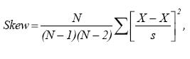
<body><![CDATA[<p align="justify"><font face="verdana" size="2"><b>Appendix A</b></font></p>     <p align="justify"><font face="verdana" size="2"><b>Formulae and computation of the Standard Precipitation Index</b></font></p>     <p align="justify"><font face="verdana" size="2">The transformation of original precipitation values (for any specified time period) into the Standard Precipitation Index has the intent of:</font></p>     <blockquote>       <p align="justify"><font face="verdana" size="2">1.&nbsp; Shifting the mean of the data to have a transformed mean of zero.</font></p>       <p align="justify"><font face="verdana" size="2">2.&nbsp; Shifting the standard deviation of the data to have a transformed value of 1.0, and</font></p>       <p align="justify"><font face="verdana" size="2">3.&nbsp;Reducing the skew existing in the data towards zero.</font></p> </blockquote>     <p align="justify"><font face="verdana" size="2"><img src="/img/revistas/atm/v18n1/a03e1.jpg">..........................................................(A1)</font></p>     <p align="justify"><font face="verdana" size="2">as an Excel function, the Mean = AVERAGE (first : last);</font></p>     <p align="justify"><font face="verdana" size="2">When these goals have been achieved, the resultant Standard Precipitation Index may be</font></p>     ]]></body>
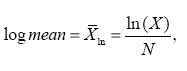
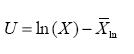
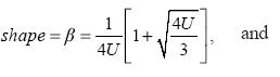
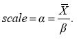
<body><![CDATA[<p align="justify"><font face="verdana" size="2"><img src="/img/revistas/atm/v18n1/a03e2.jpg">............................................................(A2)</font></p>     <p align="justify"><font face="verdana" size="2">as an Excel function, the standard deviation = STDEVP (first : last); and</font></p>     <p align="justify"><font face="verdana" size="2"><img src="/img/revistas/atm/v18n1/a03e3.jpg">...................................(A3) </font></p>     <p align="justify"><font face="verdana" size="2">as an Excel function, the skew = SKEW(first : last).</font></p>     <p align="justify"><font face="verdana" size="2">Second, the precipitation data are transformed by the log normal (ln) and the mean of those values is computed. Those transformed values are further described by the constant U, shape and</font></p>     <p align="justify"><font face="verdana" size="2"><img src="/img/revistas/atm/v18n1/a03e4.jpg">..................................................(A4)</font></p>     <p align="justify"><font face="verdana" size="2"><img src="/img/revistas/atm/v18n1/a03e5.jpg">.............................................................(A5)</font></p>     <p align="justify"><font face="verdana" size="2"><img src="/img/revistas/atm/v18n1/a03e6.jpg">....................................(A6)</font></p>     <p align="justify"><font face="verdana" size="2"><img src="/img/revistas/atm/v18n1/a03e7.jpg">................................................................(A7)</font></p>     <p align="justify"><font face="verdana" size="2">Third, the ln values are transformed by the gamma distribution, incorporating the shape and scale values:</font></p>     ]]></body>
<body><![CDATA[<p align="justify"><font face="verdana" size="2"><img src="/img/revistas/atm/v18n1/a03e8.jpg">...........(A8)</font></p>     <p align="justify"><font face="verdana" size="2">As an Excel function, Gamma transform = GAMMADIST(<i>x</i> , <i>&beta;</i>, <i>&alpha;</i>, true).</font></p>     <p align="justify"><font face="verdana" size="2">interpretable as a standardized (or z) score with a mean of zero and standard deviation of 1.0.</font></p>     <p align="justify"><font face="verdana" size="2"><img src="/img/revistas/atm/v18n1/a03e9.jpg">.........................................(A9)</font></p>     <p align="justify"><font face="verdana" size="2">This example employs Excel spreadsheet functions, where available. Other spreadsheet programs have similar functions that produce identical values.</font></p>     <p align="justify"><font face="verdana" size="2"><img src="/img/revistas/atm/v18n1/a03e10.jpg">............................(A10)</font></p>     <p align="justify"><font face="verdana" size="2">First, the precipitation data are described as to their mean, standard deviation and skew.</font></p>     <p align="justify"><font face="verdana" size="2">Fourth, the gamma transformed values are again transformed, with different formulae according to the magnitude of the gamma transformed values:</font></p>     <p align="justify"><font face="verdana" size="2">Fifth, the Standard Precipitation Index results from the t transformations, with different formulae according to the magnitude of the gamma transformed values:</font></p>     <p align="justify"><font face="verdana" size="2">where </font></p>     ]]></body>
<body><![CDATA[<blockquote>       <p align="justify"><font face="verdana" size="2">c<sub>0</sub> = 2.515517    <br>   c<sub>1</sub> = 0.802853    <br>   c<sub>2</sub> = 0.010328    <br>   d<sub>1</sub> = 1.432788    <br>   d<sub>2</sub> = 0.189269    <br>   d<sub>3</sub> = 0.001308.</font></p> </blockquote>     <p align="justify"><font face="verdana" size="2">In the following spreadsheet example, the application of these formulae results in:</font></p>     <blockquote>       <p align="justify"><font face="verdana" size="2">1)&nbsp; The January precipitation mean is adjusted from 54.42 to SPI mean of 0.01,</font></p>       ]]></body>
<body><![CDATA[<p align="justify"><font face="verdana" size="2">2)&nbsp;the standard deviation is adjusted from 36.35 to 1.00 and</font></p>       <p align="justify"><font face="verdana" size="2">3)&nbsp;the skew is reduced from 0.77 to -0.35</font></p> </blockquote>     <p align="justify"><font face="verdana" size="2">Thus, the intent of the <a href="/img/revistas/atm/v18n1/a03a1.jpg" target="_blank">Standard Precipitation Index calculation</a> has been satisfied.</font></p>     <p align="justify"><font face="verdana" size="2">&nbsp;</font></p>     <p align="justify"><font face="verdana" size="2"><b>References</b></font></p>     <!-- ref --><p align="justify"><font face="verdana" size="2">Akinremi, O. O., S. M. McGinn and A. G.. Barr, 1996. Evaluation of the Palmer Drought index on the Canadian prairies. <i>J. Climate</i>, <b>9</b>, 897-905.</font>&nbsp;&nbsp;&nbsp;&nbsp;&nbsp;&nbsp;&nbsp;&nbsp;[&#160;<a href="javascript:void(0);" onclick="javascript: window.open('/scielo.php?script=sci_nlinks&ref=1262077&pid=S0187-6236200500010000300001&lng=','','width=640,height=500,resizable=yes,scrollbars=1,menubar=yes,');">Links</a>&#160;]<!-- end-ref --><!-- ref --><p align="justify"><font face="verdana" size="2">Anctil, F.,   W. Larouche, A. A.Viau and L. E. Parent, 2002. Exploration of the standardized precipitation index with regional analysis. <i>Canadian J. Soil Science</i>, <b>82</b>, 115-125.</font>&nbsp;&nbsp;&nbsp;&nbsp;&nbsp;&nbsp;&nbsp;&nbsp;[&#160;<a href="javascript:void(0);" onclick="javascript: window.open('/scielo.php?script=sci_nlinks&ref=1262078&pid=S0187-6236200500010000300002&lng=','','width=640,height=500,resizable=yes,scrollbars=1,menubar=yes,');">Links</a>&#160;]<!-- end-ref --><!-- ref --><p align="justify"><font face="verdana" size="2">Barlow, M., S. Nigam and E. H. Berbery, 1998. Evolution of the North American monsoon system. <i>J. Climate</i>, <b>11</b>, 2238-2257.</font>&nbsp;&nbsp;&nbsp;&nbsp;&nbsp;&nbsp;&nbsp;&nbsp;[&#160;<a href="javascript:void(0);" onclick="javascript: window.open('/scielo.php?script=sci_nlinks&ref=1262079&pid=S0187-6236200500010000300003&lng=','','width=640,height=500,resizable=yes,scrollbars=1,menubar=yes,');">Links</a>&#160;]<!-- end-ref --><!-- ref --><p align="justify"><font face="verdana" size="2">Bob&eacute;e, Bernard and Ashkar and Fahim, 1991. <i>The Gamma Family and Derived Distributions Applied in Hydrology</i>. Littleton, Colorado, Water Resources Publications.</font>&nbsp;&nbsp;&nbsp;&nbsp;&nbsp;&nbsp;&nbsp;&nbsp;[&#160;<a href="javascript:void(0);" onclick="javascript: window.open('/scielo.php?script=sci_nlinks&ref=1262080&pid=S0187-6236200500010000300004&lng=','','width=640,height=500,resizable=yes,scrollbars=1,menubar=yes,');">Links</a>&#160;]<!-- end-ref --><!-- ref --><p align="justify"><font face="verdana" size="2">Bordi, I., S. Frigio, P. Parenti, A. Speranza, and A. Sutera, 2001. The analysis of the Standardized Precipitation Index in the Mediterranean area: large-scale patterns. <i>Annali Di Geofisica</i>, <b>44</b>, 965-978.</font>&nbsp;&nbsp;&nbsp;&nbsp;&nbsp;&nbsp;&nbsp;&nbsp;[&#160;<a href="javascript:void(0);" onclick="javascript: window.open('/scielo.php?script=sci_nlinks&ref=1262081&pid=S0187-6236200500010000300005&lng=','','width=640,height=500,resizable=yes,scrollbars=1,menubar=yes,');">Links</a>&#160;]<!-- end-ref --><!-- ref --><p align="justify"><font face="verdana" size="2">Bordi, I. and A. Sutera, 2001. Fifty years of precipitation: Some spatially remote teleconnnections. <i>Water Resources Management</i>, <b>15</b>, 247-280.</font>&nbsp;&nbsp;&nbsp;&nbsp;&nbsp;&nbsp;&nbsp;&nbsp;[&#160;<a href="javascript:void(0);" onclick="javascript: window.open('/scielo.php?script=sci_nlinks&ref=1262082&pid=S0187-6236200500010000300006&lng=','','width=640,height=500,resizable=yes,scrollbars=1,menubar=yes,');">Links</a>&#160;]<!-- end-ref --><!-- ref --><p align="justify"><font face="verdana" size="2">Brown, D. G., D. P. Lusch and K. A. Duda, 1998. Supervised classification of types of glaciated landscapes using digital elevation data. <i>Geomorphology</i>, <b>21</b>, 233-250.</font>&nbsp;&nbsp;&nbsp;&nbsp;&nbsp;&nbsp;&nbsp;&nbsp;[&#160;<a href="javascript:void(0);" onclick="javascript: window.open('/scielo.php?script=sci_nlinks&ref=1262083&pid=S0187-6236200500010000300007&lng=','','width=640,height=500,resizable=yes,scrollbars=1,menubar=yes,');">Links</a>&#160;]<!-- end-ref --><!-- ref --><p align="justify"><font face="verdana" size="2">Clark Labs., 1999. <i>Guide to GIS and Image Processing</i>. Worcester, Mass., Clark University.</font>&nbsp;&nbsp;&nbsp;&nbsp;&nbsp;&nbsp;&nbsp;&nbsp;[&#160;<a href="javascript:void(0);" onclick="javascript: window.open('/scielo.php?script=sci_nlinks&ref=1262084&pid=S0187-6236200500010000300008&lng=','','width=640,height=500,resizable=yes,scrollbars=1,menubar=yes,');">Links</a>&#160;]<!-- end-ref --><!-- ref --><p align="justify"><font face="verdana" size="2">Cavazos, T. and S. Hastenrath, 1990. Convection and Rainfall over Mexico and Their Modulation by the Southern Oscillation. <i>Int. J. Climatol.</i>, <b>10</b>, 377-386.</font>&nbsp;&nbsp;&nbsp;&nbsp;&nbsp;&nbsp;&nbsp;&nbsp;[&#160;<a href="javascript:void(0);" onclick="javascript: window.open('/scielo.php?script=sci_nlinks&ref=1262085&pid=S0187-6236200500010000300009&lng=','','width=640,height=500,resizable=yes,scrollbars=1,menubar=yes,');">Links</a>&#160;]<!-- end-ref --><!-- ref --><p align="justify"><font face="verdana" size="2">Douglas, M. W., R. A.Maddox, K. Howard and S. Reyes, 1993. The Mexican Monsoon. <i>J. Climate</i>, <b>6</b>, 1665-1677.</font>&nbsp;&nbsp;&nbsp;&nbsp;&nbsp;&nbsp;&nbsp;&nbsp;[&#160;<a href="javascript:void(0);" onclick="javascript: window.open('/scielo.php?script=sci_nlinks&ref=1262086&pid=S0187-6236200500010000300010&lng=','','width=640,height=500,resizable=yes,scrollbars=1,menubar=yes,');">Links</a>&#160;]<!-- end-ref --><!-- ref --><p align="justify"><font face="verdana" size="2">Edwards, D. C. and T. B. McKee, 1997. <i>Characteristics of 20th Century Drought in the United States at Multiple Time Scales</i>. Fort Collins, Colorado, Department of Atmospheric Science, Colorado State University.</font>&nbsp;&nbsp;&nbsp;&nbsp;&nbsp;&nbsp;&nbsp;&nbsp;[&#160;<a href="javascript:void(0);" onclick="javascript: window.open('/scielo.php?script=sci_nlinks&ref=1262087&pid=S0187-6236200500010000300011&lng=','','width=640,height=500,resizable=yes,scrollbars=1,menubar=yes,');">Links</a>&#160;]<!-- end-ref --><!-- ref --><p align="justify"><font face="verdana" size="2">ERIC II, 2000. Extractor r&aacute;pido de informaci&oacute;n climatol&oacute;gica. Jiutepec, Morelos, Instituto Mexicano de Tecnolog&iacute;a del Agua.</font>&nbsp;&nbsp;&nbsp;&nbsp;&nbsp;&nbsp;&nbsp;&nbsp;[&#160;<a href="javascript:void(0);" onclick="javascript: window.open('/scielo.php?script=sci_nlinks&ref=1262088&pid=S0187-6236200500010000300012&lng=','','width=640,height=500,resizable=yes,scrollbars=1,menubar=yes,');">Links</a>&#160;]<!-- end-ref --><!-- ref --><p align="justify"><font face="verdana" size="2">Fern&aacute;ndez, H. W. and B. Fern&aacute;ndez, 2002. The influence of ENSO in the precipitation regime in southern South America. <i>Ingenier&iacute;a Hidr&aacute;ulica en M&eacute;xico</i>, <b>17</b>, 5-16.</font>&nbsp;&nbsp;&nbsp;&nbsp;&nbsp;&nbsp;&nbsp;&nbsp;[&#160;<a href="javascript:void(0);" onclick="javascript: window.open('/scielo.php?script=sci_nlinks&ref=1262089&pid=S0187-6236200500010000300013&lng=','','width=640,height=500,resizable=yes,scrollbars=1,menubar=yes,');">Links</a>&#160;]<!-- end-ref --><!-- ref --><p align="justify"><font face="verdana" size="2">Fisher, W. D., 1958. On Grouping for Maximum Homogeneity. <i>J. American Statistical Association</i>, <b>53</b>, 789-798.</font>&nbsp;&nbsp;&nbsp;&nbsp;&nbsp;&nbsp;&nbsp;&nbsp;[&#160;<a href="javascript:void(0);" onclick="javascript: window.open('/scielo.php?script=sci_nlinks&ref=1262090&pid=S0187-6236200500010000300014&lng=','','width=640,height=500,resizable=yes,scrollbars=1,menubar=yes,');">Links</a>&#160;]<!-- end-ref --><!-- ref --><p align="justify"><font face="verdana" size="2">Fraley, C. and A. E. Raftery, 2002. Model-based clustering, discriminant analysis, and density estimation.<i> Journal of the American Statistical Association</i>, <b>97</b>, 611-631.</font>&nbsp;&nbsp;&nbsp;&nbsp;&nbsp;&nbsp;&nbsp;&nbsp;[&#160;<a href="javascript:void(0);" onclick="javascript: window.open('/scielo.php?script=sci_nlinks&ref=1262091&pid=S0187-6236200500010000300015&lng=','','width=640,height=500,resizable=yes,scrollbars=1,menubar=yes,');">Links</a>&#160;]<!-- end-ref --><!-- ref --><p align="justify"><font face="verdana" size="2">Garc&iacute;a, E., 1981. <i>Modificaciones al Sistema de Clasificaci&oacute;n Clim&aacute;tica de K&ouml;ppen (para adoptarlo a las condiciones de la Rep&uacute;blica Mexicana)</i>. 3rd ed. Offset Larios, M&eacute;xico, D. F.</font>&nbsp;&nbsp;&nbsp;&nbsp;&nbsp;&nbsp;&nbsp;&nbsp;[&#160;<a href="javascript:void(0);" onclick="javascript: window.open('/scielo.php?script=sci_nlinks&ref=1262092&pid=S0187-6236200500010000300016&lng=','','width=640,height=500,resizable=yes,scrollbars=1,menubar=yes,');">Links</a>&#160;]<!-- end-ref --><!-- ref --><p align="justify"><font face="verdana" size="2">Garc&iacute;a, E., R. Vidal, M. D. Cardoso and M. E. Hern&aacute;ndez, 1983. <i>Las Regiones Clim&aacute;ticas de M&eacute;xico. In Memoria del IX Congreso Nacional de Geograf&iacute;a</i>. Tomo I:123-130. Guadalajara, Jalisco.</font>&nbsp;&nbsp;&nbsp;&nbsp;&nbsp;&nbsp;&nbsp;&nbsp;[&#160;<a href="javascript:void(0);" onclick="javascript: window.open('/scielo.php?script=sci_nlinks&ref=1262093&pid=S0187-6236200500010000300017&lng=','','width=640,height=500,resizable=yes,scrollbars=1,menubar=yes,');">Links</a>&#160;]<!-- end-ref --><!-- ref --><p align="justify"><font face="verdana" size="2">Garc&iacute;a, E., R. Vidal and M. E. Hern&aacute;ndez, 1990. <i>Las Regiones Clim&aacute;ticas de M&eacute;xico</i>. In Garc&iacute;a de Fuentes, Ana. Editora. <i>Atlas Nacional de M&eacute;xico</i>, UNAM, Instituto de Geograf&iacute;a. Vol. 2 Cap. IV No. 10 Map at 1:12,000,000. M&eacute;xico DF</font>&nbsp;&nbsp;&nbsp;&nbsp;&nbsp;&nbsp;&nbsp;&nbsp;[&#160;<a href="javascript:void(0);" onclick="javascript: window.open('/scielo.php?script=sci_nlinks&ref=1262094&pid=S0187-6236200500010000300018&lng=','','width=640,height=500,resizable=yes,scrollbars=1,menubar=yes,');">Links</a>&#160;]<!-- end-ref --><!-- ref --><p align="justify"><font face="verdana" size="2">Garc&iacute;a, E., R. Vidal, L. M. Tamayo, T. Reyna, R. S&aacute;nchez, M. Soto and E. Soto, 1974. <i>Precipitaci&oacute;n de lluvia en la Rep&uacute;blica Mexicana y evaluaci&oacute;n de su probabilidad</i>, CETENAL (Comisi&oacute;n de Estudios del Territorio Nacional, Secretar&iacute;a de la Presidencia de M&eacute;xico), 32 volumes.</font>&nbsp;&nbsp;&nbsp;&nbsp;&nbsp;&nbsp;&nbsp;&nbsp;[&#160;<a href="javascript:void(0);" onclick="javascript: window.open('/scielo.php?script=sci_nlinks&ref=1262095&pid=S0187-6236200500010000300019&lng=','','width=640,height=500,resizable=yes,scrollbars=1,menubar=yes,');">Links</a>&#160;]<!-- end-ref --><!-- ref --><p align="justify"><font face="verdana" size="2">Global Historical Climate Network (GHCN), 2000. <i>Datafile access to historical world precipitation data</i>. Available on line at <a href="http://lwf.ncdc.noaa.gov/cgi-bin/res40.pl" target="_blank"><i>http://lwf.ncdc.noaa.gov/cgi-bin/res40.pl</i></a>. Ashville, N.C.</font>&nbsp;&nbsp;&nbsp;&nbsp;&nbsp;&nbsp;&nbsp;&nbsp;[&#160;<a href="javascript:void(0);" onclick="javascript: window.open('/scielo.php?script=sci_nlinks&ref=1262096&pid=S0187-6236200500010000300020&lng=','','width=640,height=500,resizable=yes,scrollbars=1,menubar=yes,');">Links</a>&#160;]<!-- end-ref --><!-- ref --><p align="justify"><font face="verdana" size="2">Golden Software, 1999. <i>Surfer 7 User's Guide</i>. Golden, Colorado, Golden Software, Inc.</font>&nbsp;&nbsp;&nbsp;&nbsp;&nbsp;&nbsp;&nbsp;&nbsp;[&#160;<a href="javascript:void(0);" onclick="javascript: window.open('/scielo.php?script=sci_nlinks&ref=1262097&pid=S0187-6236200500010000300021&lng=','','width=640,height=500,resizable=yes,scrollbars=1,menubar=yes,');">Links</a>&#160;]<!-- end-ref --><!-- ref --><p align="justify"><font face="verdana" size="2">Guttman, N. B., 1999. Accepting the standardized precipitation index: A calculation algorithm. J. <i>American Water Resources Association</i>, <b>35</b>, 311-322.</font>&nbsp;&nbsp;&nbsp;&nbsp;&nbsp;&nbsp;&nbsp;&nbsp;[&#160;<a href="javascript:void(0);" onclick="javascript: window.open('/scielo.php?script=sci_nlinks&ref=1262098&pid=S0187-6236200500010000300022&lng=','','width=640,height=500,resizable=yes,scrollbars=1,menubar=yes,');">Links</a>&#160;]<!-- end-ref --><!-- ref --><p align="justify"><font face="verdana" size="2">Guttman, N. B., J. R. Wallis and J. R. M. Hosking, 1992. Spatial Comparability of the Palmer Drought Severity Index. <i>Water Resources Bull.</i>, <b>28</b>, 1111-1119.</font>&nbsp;&nbsp;&nbsp;&nbsp;&nbsp;&nbsp;&nbsp;&nbsp;[&#160;<a href="javascript:void(0);" onclick="javascript: window.open('/scielo.php?script=sci_nlinks&ref=1262099&pid=S0187-6236200500010000300023&lng=','','width=640,height=500,resizable=yes,scrollbars=1,menubar=yes,');">Links</a>&#160;]<!-- end-ref --><!-- ref --><p align="justify"><font face="verdana" size="2">Hayes, M. J., M. D. Svoboda, D. A. Wilhite and O. V. Vanyarkho, 1999. Monitoring the 1996 drought using the standardized precipitation index. <i>Bull. Amer. Meteorol. Soc</i>., <b>80</b>, 429-438.</font>&nbsp;&nbsp;&nbsp;&nbsp;&nbsp;&nbsp;&nbsp;&nbsp;[&#160;<a href="javascript:void(0);" onclick="javascript: window.open('/scielo.php?script=sci_nlinks&ref=1262100&pid=S0187-6236200500010000300024&lng=','','width=640,height=500,resizable=yes,scrollbars=1,menubar=yes,');">Links</a>&#160;]<!-- end-ref --><!-- ref --><p align="justify"><font face="verdana" size="2">Herrero, J. and M. A. Casterad, 1999. Using satellite and other data to estimate the annual water demand of an irrigation district. <i>Environmental Monitoring Assessment</i>, <b>55</b>, 305-317.</font>&nbsp;&nbsp;&nbsp;&nbsp;&nbsp;&nbsp;&nbsp;&nbsp;[&#160;<a href="javascript:void(0);" onclick="javascript: window.open('/scielo.php?script=sci_nlinks&ref=1262101&pid=S0187-6236200500010000300025&lng=','','width=640,height=500,resizable=yes,scrollbars=1,menubar=yes,');">Links</a>&#160;]<!-- end-ref --><!-- ref --><p align="justify"><font face="verdana" size="2">Higgins, R. W., Y. Chen and A. V. Douglas, 1999. Interannual variability of the North American warm season precipitation regime.<i> J. Climate</i>, <b>12</b>, 653-680.</font>&nbsp;&nbsp;&nbsp;&nbsp;&nbsp;&nbsp;&nbsp;&nbsp;[&#160;<a href="javascript:void(0);" onclick="javascript: window.open('/scielo.php?script=sci_nlinks&ref=1262102&pid=S0187-6236200500010000300026&lng=','','width=640,height=500,resizable=yes,scrollbars=1,menubar=yes,');">Links</a>&#160;]<!-- end-ref --><!-- ref --><p align="justify"><font face="verdana" size="2">Jim&eacute;nez, L. O. and D. A. Landgrebe, 1998. Supervised classification in high-dimensional space: Geometrical, statistical, and asymptotical properties of multivariate data. <i>IEEE Transactions on Systems, Man and Cybernetics Part C- Applications and Reviews</i>, <b>28</b>, 39-54.</font>&nbsp;&nbsp;&nbsp;&nbsp;&nbsp;&nbsp;&nbsp;&nbsp;[&#160;<a href="javascript:void(0);" onclick="javascript: window.open('/scielo.php?script=sci_nlinks&ref=1262103&pid=S0187-6236200500010000300027&lng=','','width=640,height=500,resizable=yes,scrollbars=1,menubar=yes,');">Links</a>&#160;]<!-- end-ref --><!-- ref --><p align="justify"><font face="verdana" size="2">Keyantash, J. and J. A. Dracup, 2002. The quantification of drought: An evaluation of drought indices. <i>Bull. Amer. Meteorol. Soc.</i>, <b>83</b>, 1167-1180.</font>&nbsp;&nbsp;&nbsp;&nbsp;&nbsp;&nbsp;&nbsp;&nbsp;[&#160;<a href="javascript:void(0);" onclick="javascript: window.open('/scielo.php?script=sci_nlinks&ref=1262104&pid=S0187-6236200500010000300028&lng=','','width=640,height=500,resizable=yes,scrollbars=1,menubar=yes,');">Links</a>&#160;]<!-- end-ref --><!-- ref --><p align="justify"><font face="verdana" size="2">Lahey Computer Systems, 1998. Lahey-Fujitsu Fortran 95 Language Reference: Revision D. Incline Village, Nevada: Lahey Computer Systems, Inc.</font>&nbsp;&nbsp;&nbsp;&nbsp;&nbsp;&nbsp;&nbsp;&nbsp;[&#160;<a href="javascript:void(0);" onclick="javascript: window.open('/scielo.php?script=sci_nlinks&ref=1262105&pid=S0187-6236200500010000300029&lng=','','width=640,height=500,resizable=yes,scrollbars=1,menubar=yes,');">Links</a>&#160;]<!-- end-ref --><!-- ref --><p align="justify"><font face="verdana" size="2">Lauver, C. L., 1997. Mapping species diversity patterns in the Kansas shortgrass region by integrating remote sensing and vegetation analysis. <i>J. Vegetation Science</i>, <b>8</b>, 387-394.</font>&nbsp;&nbsp;&nbsp;&nbsp;&nbsp;&nbsp;&nbsp;&nbsp;[&#160;<a href="javascript:void(0);" onclick="javascript: window.open('/scielo.php?script=sci_nlinks&ref=1262106&pid=S0187-6236200500010000300030&lng=','','width=640,height=500,resizable=yes,scrollbars=1,menubar=yes,');">Links</a>&#160;]<!-- end-ref --><!-- ref --><p align="justify"><font face="verdana" size="2">Lloyd-Hughes, B. and M. A. Saunders, 2002. A drought climatology for Europe. <i>Int. J. Climatol.</i>, <b>22</b>, 1571-1592.</font>&nbsp;&nbsp;&nbsp;&nbsp;&nbsp;&nbsp;&nbsp;&nbsp;[&#160;<a href="javascript:void(0);" onclick="javascript: window.open('/scielo.php?script=sci_nlinks&ref=1262107&pid=S0187-6236200500010000300031&lng=','','width=640,height=500,resizable=yes,scrollbars=1,menubar=yes,');">Links</a>&#160;]<!-- end-ref --><!-- ref --><p align="justify"><font face="verdana" size="2">Love, B. C., 2002. Comparing supervised and unsupervised category learning. <i>Psychonomic Bulletin and Review</i>, <b>9</b>, 829-835.</font>&nbsp;&nbsp;&nbsp;&nbsp;&nbsp;&nbsp;&nbsp;&nbsp;[&#160;<a href="javascript:void(0);" onclick="javascript: window.open('/scielo.php?script=sci_nlinks&ref=1262108&pid=S0187-6236200500010000300032&lng=','','width=640,height=500,resizable=yes,scrollbars=1,menubar=yes,');">Links</a>&#160;]<!-- end-ref --><!-- ref --><p align="justify"><font face="verdana" size="2">Maga&ntilde;a, V. E., J. L. P&eacute;rez, J. L. V&aacute;zquez, E. Carrisoza and J. P&eacute;rez, 1999. El Ni&ntilde;o y el clima. In <i>Los Impactos de El Ni&ntilde;o en M&eacute;xico</i>. M&eacute;xico, D. F., Secretar&iacute;a de Gobernaci&oacute;n.</font>&nbsp;&nbsp;&nbsp;&nbsp;&nbsp;&nbsp;&nbsp;&nbsp;[&#160;<a href="javascript:void(0);" onclick="javascript: window.open('/scielo.php?script=sci_nlinks&ref=1262109&pid=S0187-6236200500010000300033&lng=','','width=640,height=500,resizable=yes,scrollbars=1,menubar=yes,');">Links</a>&#160;]<!-- end-ref --><!-- ref --><p align="justify"><font face="verdana" size="2">McKee, T. B., N. J. Doesken and J. Kleist, 1993. <i>Drought monitoring with multiple timescales</i>. Paper presented at the Preprints, Eighth Conference on Applied Climatology, Anaheim, California.</font>&nbsp;&nbsp;&nbsp;&nbsp;&nbsp;&nbsp;&nbsp;&nbsp;[&#160;<a href="javascript:void(0);" onclick="javascript: window.open('/scielo.php?script=sci_nlinks&ref=1262110&pid=S0187-6236200500010000300034&lng=','','width=640,height=500,resizable=yes,scrollbars=1,menubar=yes,');">Links</a>&#160;]<!-- end-ref --><!-- ref --><p align="justify"><font face="verdana" size="2">Mosi&ntilde;o, A. P. and E. Garc&iacute;a, 1974. The climate of M&eacute;xico. In: R. A. Bryson and F. K. Hare (Eds.), <i>The Climates of North America, World Survey of Climatology</i>, 345-404. Amsterdam, Elsevier.</font>&nbsp;&nbsp;&nbsp;&nbsp;&nbsp;&nbsp;&nbsp;&nbsp;[&#160;<a href="javascript:void(0);" onclick="javascript: window.open('/scielo.php?script=sci_nlinks&ref=1262111&pid=S0187-6236200500010000300035&lng=','','width=640,height=500,resizable=yes,scrollbars=1,menubar=yes,');">Links</a>&#160;]<!-- end-ref --><!-- ref --><p align="justify"><font face="verdana" size="2">Przybyszewska, A., J. Pniewski and T. Szoplik, 1999. Supervised classification of Lobez forest area in Landsat images. <i>Optica Applicata</i>, <b>29</b>, 529-542.</font>&nbsp;&nbsp;&nbsp;&nbsp;&nbsp;&nbsp;&nbsp;&nbsp;[&#160;<a href="javascript:void(0);" onclick="javascript: window.open('/scielo.php?script=sci_nlinks&ref=1262112&pid=S0187-6236200500010000300036&lng=','','width=640,height=500,resizable=yes,scrollbars=1,menubar=yes,');">Links</a>&#160;]<!-- end-ref --><!-- ref --><p align="justify"><font face="verdana" size="2">Quintas, I., 2000. ERIC II, <i>Documentaci&oacute;n de la base de datos climatol&oacute;gica y del programa extractor</i>. Progreso, Morelos, Instituto Mexicano de Tecnolog&iacute;a del Agua.</font>&nbsp;&nbsp;&nbsp;&nbsp;&nbsp;&nbsp;&nbsp;&nbsp;[&#160;<a href="javascript:void(0);" onclick="javascript: window.open('/scielo.php?script=sci_nlinks&ref=1262113&pid=S0187-6236200500010000300037&lng=','','width=640,height=500,resizable=yes,scrollbars=1,menubar=yes,');">Links</a>&#160;]<!-- end-ref --><!-- ref --><p align="justify"><font face="verdana" size="2">Rughooputh, S., S. Oodit, S. Persand, K. Golap and R. Somanah, 2000. A new tool for handling astronomical images. <i>Astrophysics and Space Science</i>, <b>273</b>, 245-256.</font>&nbsp;&nbsp;&nbsp;&nbsp;&nbsp;&nbsp;&nbsp;&nbsp;[&#160;<a href="javascript:void(0);" onclick="javascript: window.open('/scielo.php?script=sci_nlinks&ref=1262114&pid=S0187-6236200500010000300038&lng=','','width=640,height=500,resizable=yes,scrollbars=1,menubar=yes,');">Links</a>&#160;]<!-- end-ref --><!-- ref --><p align="justify"><font face="verdana" size="2">Seiler, R. A., M. Hayes and L. Bressan, 2002. Using the standardized precipitation index for flood risk monitoring. <i>Int. J. Climatol.</i>, <b>22</b>, 1365-1376.</font>&nbsp;&nbsp;&nbsp;&nbsp;&nbsp;&nbsp;&nbsp;&nbsp;[&#160;<a href="javascript:void(0);" onclick="javascript: window.open('/scielo.php?script=sci_nlinks&ref=1262115&pid=S0187-6236200500010000300039&lng=','','width=640,height=500,resizable=yes,scrollbars=1,menubar=yes,');">Links</a>&#160;]<!-- end-ref --><!-- ref --><p align="justify"><font face="verdana" size="2">Sims, A. P., D. D. S. Niyogi and S. Raman, 2002. Adopting drought indices for estimating soil moisture: A North Carolina case study. <i>Geophysical Research Letters</i>, <b>29</b>, art. no. 1183.</font>&nbsp;&nbsp;&nbsp;&nbsp;&nbsp;&nbsp;&nbsp;&nbsp;[&#160;<a href="javascript:void(0);" onclick="javascript: window.open('/scielo.php?script=sci_nlinks&ref=1262116&pid=S0187-6236200500010000300040&lng=','','width=640,height=500,resizable=yes,scrollbars=1,menubar=yes,');">Links</a>&#160;]<!-- end-ref --><!-- ref --><p align="justify"><font face="verdana" size="2">Yamoah, C. F., G. E. Varvel, C. A. Francis and W. J. Waltman, 1998. Weather and management impact on crop yield variability in rotations. <i>J. Production Agriculture</i>, <b>11</b>, 219-225.</font>&nbsp;&nbsp;&nbsp;&nbsp;&nbsp;&nbsp;&nbsp;&nbsp;[&#160;<a href="javascript:void(0);" onclick="javascript: window.open('/scielo.php?script=sci_nlinks&ref=1262117&pid=S0187-6236200500010000300041&lng=','','width=640,height=500,resizable=yes,scrollbars=1,menubar=yes,');">Links</a>&#160;]<!-- end-ref --><!-- ref --><p align="justify"><font face="verdana" size="2">Yamoah, C. F., D. T. Walters, C. A. Shapiro, C. A. Francis and M. J. Hayes, 2000. Standardized precipitation index and nitrogen rate effects on crop yields and risk distribution in maize. <i>Agriculture Ecosystems and Environment</i>, <b>80</b>, 113-120.</font>&nbsp;&nbsp;&nbsp;&nbsp;&nbsp;&nbsp;&nbsp;&nbsp;[&#160;<a href="javascript:void(0);" onclick="javascript: window.open('/scielo.php?script=sci_nlinks&ref=1262118&pid=S0187-6236200500010000300042&lng=','','width=640,height=500,resizable=yes,scrollbars=1,menubar=yes,');">Links</a>&#160;]<!-- end-ref --><!-- ref --><p align="justify"><font face="verdana" size="2">Yu, B. and J. M. Wallace, 2000. The principal mode of interannual variability of the North American Monsoon System. <i>J. Climate</i>, <b>13</b>, 2794-2800.</font>&nbsp;&nbsp;&nbsp;&nbsp;&nbsp;&nbsp;&nbsp;&nbsp;[&#160;<a href="javascript:void(0);" onclick="javascript: window.open('/scielo.php?script=sci_nlinks&ref=1262119&pid=S0187-6236200500010000300043&lng=','','width=640,height=500,resizable=yes,scrollbars=1,menubar=yes,');">Links</a>&#160;]<!-- end-ref --> ]]></body><back>
<ref-list>
<ref id="B1">
<nlm-citation citation-type="journal">
<person-group person-group-type="author">
<name>
<surname><![CDATA[Akinremi]]></surname>
<given-names><![CDATA[O. O.]]></given-names>
</name>
<name>
<surname><![CDATA[McGinn]]></surname>
<given-names><![CDATA[S. M.]]></given-names>
</name>
<name>
<surname><![CDATA[Barr]]></surname>
<given-names><![CDATA[A. G.]]></given-names>
</name>
</person-group>
<article-title xml:lang="en"><![CDATA[Evaluation of the Palmer Drought index on the Canadian prairies]]></article-title>
<source><![CDATA[J. Climate]]></source>
<year>1996</year>
<numero>9</numero>
<issue>9</issue>
<page-range>897-905</page-range></nlm-citation>
</ref>
<ref id="B2">
<nlm-citation citation-type="journal">
<person-group person-group-type="author">
<name>
<surname><![CDATA[Anctil]]></surname>
<given-names><![CDATA[F.]]></given-names>
</name>
<name>
<surname><![CDATA[Larouche]]></surname>
<given-names><![CDATA[W.]]></given-names>
</name>
<name>
<surname><![CDATA[Viau]]></surname>
<given-names><![CDATA[A. A.]]></given-names>
</name>
<name>
<surname><![CDATA[Parent]]></surname>
<given-names><![CDATA[L. E.]]></given-names>
</name>
</person-group>
<article-title xml:lang="en"><![CDATA[Exploration of the standardized precipitation index with regional analysis]]></article-title>
<source><![CDATA[Canadian J. Soil Science]]></source>
<year>2002</year>
<numero>82</numero>
<issue>82</issue>
<page-range>115-125</page-range></nlm-citation>
</ref>
<ref id="B3">
<nlm-citation citation-type="journal">
<person-group person-group-type="author">
<name>
<surname><![CDATA[Barlow]]></surname>
<given-names><![CDATA[M.]]></given-names>
</name>
<name>
<surname><![CDATA[Nigam]]></surname>
<given-names><![CDATA[S.]]></given-names>
</name>
<name>
<surname><![CDATA[Berbery]]></surname>
<given-names><![CDATA[E. H.]]></given-names>
</name>
</person-group>
<article-title xml:lang="en"><![CDATA[Evolution of the North American monsoon system]]></article-title>
<source><![CDATA[J. Climate]]></source>
<year>1998</year>
<numero>11</numero>
<issue>11</issue>
<page-range>2238-2257</page-range></nlm-citation>
</ref>
<ref id="B4">
<nlm-citation citation-type="book">
<person-group person-group-type="author">
<name>
<surname><![CDATA[Bobée]]></surname>
</name>
<name>
<surname><![CDATA[Bernard]]></surname>
</name>
<name>
<surname><![CDATA[Ashkar]]></surname>
</name>
<name>
<surname><![CDATA[Fahim]]></surname>
</name>
</person-group>
<source><![CDATA[The Gamma Family and Derived Distributions Applied in Hydrology]]></source>
<year>1991</year>
<publisher-loc><![CDATA[Littleton^eColorado Colorado]]></publisher-loc>
<publisher-name><![CDATA[Water Resources Publications]]></publisher-name>
</nlm-citation>
</ref>
<ref id="B5">
<nlm-citation citation-type="journal">
<person-group person-group-type="author">
<name>
<surname><![CDATA[Bordi]]></surname>
<given-names><![CDATA[I.]]></given-names>
</name>
<name>
<surname><![CDATA[Frigio]]></surname>
<given-names><![CDATA[S.]]></given-names>
</name>
<name>
<surname><![CDATA[Parenti]]></surname>
<given-names><![CDATA[P.]]></given-names>
</name>
<name>
<surname><![CDATA[Speranza]]></surname>
<given-names><![CDATA[A.]]></given-names>
</name>
<name>
<surname><![CDATA[Sutera]]></surname>
<given-names><![CDATA[A.]]></given-names>
</name>
</person-group>
<article-title xml:lang="en"><![CDATA[The analysis of the Standardized Precipitation Index in the Mediterranean area: large-scale patterns]]></article-title>
<source><![CDATA[Annali Di Geofisica]]></source>
<year>2001</year>
<numero>44</numero>
<issue>44</issue>
<page-range>965-978</page-range></nlm-citation>
</ref>
<ref id="B6">
<nlm-citation citation-type="journal">
<person-group person-group-type="author">
<name>
<surname><![CDATA[Bordi]]></surname>
<given-names><![CDATA[I.]]></given-names>
</name>
<name>
<surname><![CDATA[Sutera]]></surname>
<given-names><![CDATA[A.]]></given-names>
</name>
</person-group>
<article-title xml:lang="en"><![CDATA[Fifty years of precipitation: Some spatially remote teleconnnections]]></article-title>
<source><![CDATA[Water Resources Management]]></source>
<year>2001</year>
<numero>15</numero>
<issue>15</issue>
<page-range>247-280</page-range></nlm-citation>
</ref>
<ref id="B7">
<nlm-citation citation-type="journal">
<person-group person-group-type="author">
<name>
<surname><![CDATA[Brown]]></surname>
<given-names><![CDATA[D. G.]]></given-names>
</name>
<name>
<surname><![CDATA[Lusch]]></surname>
<given-names><![CDATA[D. P.]]></given-names>
</name>
<name>
<surname><![CDATA[Duda]]></surname>
<given-names><![CDATA[K. A.]]></given-names>
</name>
</person-group>
<article-title xml:lang="en"><![CDATA[Supervised classification of types of glaciated landscapes using digital elevation data]]></article-title>
<source><![CDATA[Geomorphology]]></source>
<year>1998</year>
<numero>21</numero>
<issue>21</issue>
<page-range>233-250</page-range></nlm-citation>
</ref>
<ref id="B8">
<nlm-citation citation-type="book">
<collab>Clark Labs.</collab>
<source><![CDATA[Guide to GIS and Image Processing]]></source>
<year>1999</year>
<publisher-loc><![CDATA[Worcester^eMass. Mass.]]></publisher-loc>
<publisher-name><![CDATA[Clark University]]></publisher-name>
</nlm-citation>
</ref>
<ref id="B9">
<nlm-citation citation-type="journal">
<person-group person-group-type="author">
<name>
<surname><![CDATA[Cavazos]]></surname>
<given-names><![CDATA[T.]]></given-names>
</name>
<name>
<surname><![CDATA[Hastenrath]]></surname>
<given-names><![CDATA[S.]]></given-names>
</name>
</person-group>
<article-title xml:lang="en"><![CDATA[Convection and Rainfall over Mexico and Their Modulation by the Southern Oscillation]]></article-title>
<source><![CDATA[Int. J. Climatol.]]></source>
<year>1990</year>
<numero>10</numero>
<issue>10</issue>
<page-range>377-386</page-range></nlm-citation>
</ref>
<ref id="B10">
<nlm-citation citation-type="journal">
<person-group person-group-type="author">
<name>
<surname><![CDATA[Douglas]]></surname>
<given-names><![CDATA[M. W.]]></given-names>
</name>
<name>
<surname><![CDATA[Maddox]]></surname>
<given-names><![CDATA[R. A.]]></given-names>
</name>
<name>
<surname><![CDATA[Howard]]></surname>
<given-names><![CDATA[K.]]></given-names>
</name>
<name>
<surname><![CDATA[Reyes]]></surname>
<given-names><![CDATA[S.]]></given-names>
</name>
</person-group>
<article-title xml:lang="en"><![CDATA[The Mexican Monsoon]]></article-title>
<source><![CDATA[J. Climate]]></source>
<year>1993</year>
<numero>6</numero>
<issue>6</issue>
<page-range>1665-1677</page-range></nlm-citation>
</ref>
<ref id="B11">
<nlm-citation citation-type="book">
<person-group person-group-type="author">
<name>
<surname><![CDATA[Edwards]]></surname>
<given-names><![CDATA[D. C.]]></given-names>
</name>
<name>
<surname><![CDATA[McKee]]></surname>
<given-names><![CDATA[T. B.]]></given-names>
</name>
</person-group>
<source><![CDATA[Characteristics of 20th Century Drought in the United States at Multiple Time Scales]]></source>
<year>1997</year>
<publisher-loc><![CDATA[Fort Collins^eColorado Colorado]]></publisher-loc>
<publisher-name><![CDATA[Department of Atmospheric Science, Colorado State University]]></publisher-name>
</nlm-citation>
</ref>
<ref id="B12">
<nlm-citation citation-type="book">
<collab>ERIC II</collab>
<source><![CDATA[Extractor rápido de información climatológica]]></source>
<year>2000</year>
<publisher-loc><![CDATA[Jiutepec^eMorelos Morelos]]></publisher-loc>
<publisher-name><![CDATA[Instituto Mexicano de Tecnología del Agua]]></publisher-name>
</nlm-citation>
</ref>
<ref id="B13">
<nlm-citation citation-type="journal">
<person-group person-group-type="author">
<name>
<surname><![CDATA[Fernández]]></surname>
<given-names><![CDATA[H. W.]]></given-names>
</name>
<name>
<surname><![CDATA[Fernández]]></surname>
<given-names><![CDATA[B.]]></given-names>
</name>
</person-group>
<article-title xml:lang="en"><![CDATA[The influence of ENSO in the precipitation regime in southern South America]]></article-title>
<source><![CDATA[Ingeniería Hidráulica en México]]></source>
<year>2002</year>
<numero>17</numero>
<issue>17</issue>
<page-range>5-16</page-range></nlm-citation>
</ref>
<ref id="B14">
<nlm-citation citation-type="journal">
<person-group person-group-type="author">
<name>
<surname><![CDATA[Fisher]]></surname>
<given-names><![CDATA[W. D.]]></given-names>
</name>
</person-group>
<article-title xml:lang="en"><![CDATA[On Grouping for Maximum Homogeneity]]></article-title>
<source><![CDATA[J. American Statistical Association]]></source>
<year>1958</year>
<numero>53</numero>
<issue>53</issue>
<page-range>789-798</page-range></nlm-citation>
</ref>
<ref id="B15">
<nlm-citation citation-type="journal">
<person-group person-group-type="author">
<name>
<surname><![CDATA[Fraley]]></surname>
<given-names><![CDATA[C.]]></given-names>
</name>
<name>
<surname><![CDATA[Raftery]]></surname>
<given-names><![CDATA[A. E.]]></given-names>
</name>
</person-group>
<article-title xml:lang="en"><![CDATA[Model-based clustering, discriminant analysis, and density estimation]]></article-title>
<source><![CDATA[Journal of the American Statistical Association]]></source>
<year>2002</year>
<numero>97</numero>
<issue>97</issue>
<page-range>611-631</page-range></nlm-citation>
</ref>
<ref id="B16">
<nlm-citation citation-type="book">
<person-group person-group-type="author">
<name>
<surname><![CDATA[García]]></surname>
<given-names><![CDATA[E.]]></given-names>
</name>
</person-group>
<source><![CDATA[Modificaciones al Sistema de Clasificación Climática de Köppen (para adoptarlo a las condiciones de la República Mexicana)]]></source>
<year>1981</year>
<edition>3rd ed</edition>
<publisher-loc><![CDATA[D. F. ]]></publisher-loc>
<publisher-name><![CDATA[Offset Larios]]></publisher-name>
</nlm-citation>
</ref>
<ref id="B17">
<nlm-citation citation-type="">
<person-group person-group-type="author">
<name>
<surname><![CDATA[García]]></surname>
<given-names><![CDATA[E.]]></given-names>
</name>
<name>
<surname><![CDATA[Vidal]]></surname>
<given-names><![CDATA[R.]]></given-names>
</name>
<name>
<surname><![CDATA[Cardoso]]></surname>
<given-names><![CDATA[M. D.]]></given-names>
</name>
<name>
<surname><![CDATA[Hernández]]></surname>
<given-names><![CDATA[M. E.]]></given-names>
</name>
</person-group>
<article-title xml:lang="es"><![CDATA[Las Regiones Climáticas de México]]></article-title>
<source><![CDATA[Memoria del IX Congreso Nacional de Geografía]]></source>
<year>1983</year>
<publisher-loc><![CDATA[Guadalajara^eJalisco Jalisco]]></publisher-loc>
</nlm-citation>
</ref>
<ref id="B18">
<nlm-citation citation-type="book">
<person-group person-group-type="author">
<name>
<surname><![CDATA[García]]></surname>
<given-names><![CDATA[E.]]></given-names>
</name>
<name>
<surname><![CDATA[Vidal]]></surname>
<given-names><![CDATA[R.]]></given-names>
</name>
<name>
<surname><![CDATA[Hernández]]></surname>
<given-names><![CDATA[M. E.]]></given-names>
</name>
</person-group>
<article-title xml:lang="es"><![CDATA[Las Regiones Climáticas de México]]></article-title>
<person-group person-group-type="editor">
<name>
<surname><![CDATA[García de Fuentes]]></surname>
<given-names><![CDATA[Ana]]></given-names>
</name>
</person-group>
<source><![CDATA[Atlas Nacional de México]]></source>
<year>1990</year>
<volume>2</volume>
<publisher-loc><![CDATA[México^eDF DF]]></publisher-loc>
<publisher-name><![CDATA[UNAM, Instituto de Geografía]]></publisher-name>
</nlm-citation>
</ref>
<ref id="B19">
<nlm-citation citation-type="book">
<person-group person-group-type="author">
<name>
<surname><![CDATA[García]]></surname>
<given-names><![CDATA[E.]]></given-names>
</name>
<name>
<surname><![CDATA[Vidal]]></surname>
<given-names><![CDATA[R.]]></given-names>
</name>
<name>
<surname><![CDATA[Tamayo]]></surname>
<given-names><![CDATA[L. M.]]></given-names>
</name>
<name>
<surname><![CDATA[Reyna]]></surname>
<given-names><![CDATA[T.]]></given-names>
</name>
<name>
<surname><![CDATA[Sánchez]]></surname>
<given-names><![CDATA[R.]]></given-names>
</name>
<name>
<surname><![CDATA[Soto]]></surname>
<given-names><![CDATA[M.]]></given-names>
</name>
<name>
<surname><![CDATA[Soto]]></surname>
<given-names><![CDATA[E.]]></given-names>
</name>
</person-group>
<source><![CDATA[Precipitación de lluvia en la República Mexicana y evaluación de su probabilidad]]></source>
<year>1974</year>
<volume>32</volume>
<publisher-name><![CDATA[CETENAL (Comisión de Estudios del Territorio Nacional, Secretaría de la Presidencia de México)]]></publisher-name>
</nlm-citation>
</ref>
<ref id="B20">
<nlm-citation citation-type="">
<collab>Global Historical Climate Network</collab>
<source><![CDATA[Datafile access to historical world precipitation data]]></source>
<year>2000</year>
<publisher-loc><![CDATA[Ashville^eN.C. N.C.]]></publisher-loc>
</nlm-citation>
</ref>
<ref id="B21">
<nlm-citation citation-type="book">
<collab>Golden Software</collab>
<source><![CDATA[Surfer 7 User's Guide]]></source>
<year>1999</year>
<publisher-loc><![CDATA[Golden^eColorado Colorado]]></publisher-loc>
<publisher-name><![CDATA[Golden Software, Inc]]></publisher-name>
</nlm-citation>
</ref>
<ref id="B22">
<nlm-citation citation-type="journal">
<person-group person-group-type="author">
<name>
<surname><![CDATA[Guttman]]></surname>
<given-names><![CDATA[N. B.]]></given-names>
</name>
</person-group>
<article-title xml:lang="en"><![CDATA[Accepting the standardized precipitation index: A calculation algorithm]]></article-title>
<source><![CDATA[J. American Water Resources Association]]></source>
<year>1999</year>
<numero>35</numero>
<issue>35</issue>
<page-range>311-322</page-range></nlm-citation>
</ref>
<ref id="B23">
<nlm-citation citation-type="journal">
<person-group person-group-type="author">
<name>
<surname><![CDATA[Guttman]]></surname>
<given-names><![CDATA[N. B.]]></given-names>
</name>
<name>
<surname><![CDATA[Wallis]]></surname>
<given-names><![CDATA[J. R.]]></given-names>
</name>
<name>
<surname><![CDATA[Hosking]]></surname>
<given-names><![CDATA[J. R. M.]]></given-names>
</name>
</person-group>
<article-title xml:lang="en"><![CDATA[Spatial Comparability of the Palmer Drought Severity Index]]></article-title>
<source><![CDATA[Water Resources Bull.]]></source>
<year>1992</year>
<numero>28</numero>
<issue>28</issue>
<page-range>1111-1119</page-range></nlm-citation>
</ref>
<ref id="B24">
<nlm-citation citation-type="journal">
<person-group person-group-type="author">
<name>
<surname><![CDATA[Hayes]]></surname>
<given-names><![CDATA[M. J.]]></given-names>
</name>
<name>
<surname><![CDATA[Svoboda]]></surname>
<given-names><![CDATA[M. D.]]></given-names>
</name>
<name>
<surname><![CDATA[Wilhite]]></surname>
<given-names><![CDATA[D. A.]]></given-names>
</name>
<name>
<surname><![CDATA[Vanyarkho]]></surname>
<given-names><![CDATA[O. V.]]></given-names>
</name>
</person-group>
<source><![CDATA[Bull. Amer. Meteorol. Soc.Monitoring the 1996 drought using the standardized precipitation index]]></source>
<year>1999</year>
<numero>80</numero>
<issue>80</issue>
<page-range>429-438</page-range></nlm-citation>
</ref>
<ref id="B25">
<nlm-citation citation-type="journal">
<person-group person-group-type="author">
<name>
<surname><![CDATA[Herrero]]></surname>
<given-names><![CDATA[J.]]></given-names>
</name>
<name>
<surname><![CDATA[Casterad]]></surname>
<given-names><![CDATA[M. A.]]></given-names>
</name>
</person-group>
<article-title xml:lang="en"><![CDATA[Using satellite and other data to estimate the annual water demand of an irrigation district]]></article-title>
<source><![CDATA[Environmental Monitoring Assessment]]></source>
<year>1999</year>
<numero>55</numero>
<issue>55</issue>
<page-range>305-317</page-range></nlm-citation>
</ref>
<ref id="B26">
<nlm-citation citation-type="journal">
<person-group person-group-type="author">
<name>
<surname><![CDATA[Higgins]]></surname>
<given-names><![CDATA[R. W.]]></given-names>
</name>
<name>
<surname><![CDATA[Chen]]></surname>
<given-names><![CDATA[Y.]]></given-names>
</name>
<name>
<surname><![CDATA[Douglas]]></surname>
<given-names><![CDATA[A. V.]]></given-names>
</name>
</person-group>
<article-title xml:lang="en"><![CDATA[Interannual variability of the North American warm season precipitation regime]]></article-title>
<source><![CDATA[J. Climate]]></source>
<year>1999</year>
<numero>12</numero>
<issue>12</issue>
<page-range>653-680</page-range></nlm-citation>
</ref>
<ref id="B27">
<nlm-citation citation-type="journal">
<person-group person-group-type="author">
<name>
<surname><![CDATA[Jiménez]]></surname>
<given-names><![CDATA[L. O.]]></given-names>
</name>
<name>
<surname><![CDATA[Landgrebe]]></surname>
<given-names><![CDATA[D. A]]></given-names>
</name>
</person-group>
<article-title xml:lang="en"><![CDATA[Supervised classification in high-dimensional space: Geometrical, statistical, and asymptotical properties of multivariate data]]></article-title>
<source><![CDATA[IEEE Transactions on Systems, Man and Cybernetics Part C- Applications and Reviews]]></source>
<year>1998</year>
<numero>28</numero>
<issue>28</issue>
<page-range>39-54</page-range></nlm-citation>
</ref>
<ref id="B28">
<nlm-citation citation-type="journal">
<person-group person-group-type="author">
<name>
<surname><![CDATA[Keyantash]]></surname>
<given-names><![CDATA[J.]]></given-names>
</name>
<name>
<surname><![CDATA[Dracup]]></surname>
<given-names><![CDATA[J. A.]]></given-names>
</name>
</person-group>
<article-title xml:lang="en"><![CDATA[The quantification of drought: An evaluation of drought indices]]></article-title>
<source><![CDATA[Bull. Amer. Meteorol. Soc.]]></source>
<year>2002</year>
<numero>83</numero>
<issue>83</issue>
<page-range>1167-1180</page-range></nlm-citation>
</ref>
<ref id="B29">
<nlm-citation citation-type="book">
<collab>Lahey Computer Systems</collab>
<source><![CDATA[Lahey-Fujitsu Fortran 95 Language Reference: Revision D. Incline Village, Nevada]]></source>
<year>1998</year>
<publisher-name><![CDATA[Lahey Computer Systems, Inc.]]></publisher-name>
</nlm-citation>
</ref>
<ref id="B30">
<nlm-citation citation-type="journal">
<person-group person-group-type="author">
<name>
<surname><![CDATA[Lauver]]></surname>
<given-names><![CDATA[C. L.]]></given-names>
</name>
</person-group>
<article-title xml:lang="en"><![CDATA[Mapping species diversity patterns in the Kansas shortgrass region by integrating remote sensing and vegetation analysis]]></article-title>
<source><![CDATA[J. Vegetation Science]]></source>
<year>1997</year>
<numero>8</numero>
<issue>8</issue>
<page-range>387-394</page-range></nlm-citation>
</ref>
<ref id="B31">
<nlm-citation citation-type="journal">
<person-group person-group-type="author">
<name>
<surname><![CDATA[Lloyd-Hughes]]></surname>
<given-names><![CDATA[B.]]></given-names>
</name>
<name>
<surname><![CDATA[Saunders]]></surname>
<given-names><![CDATA[M. A.]]></given-names>
</name>
</person-group>
<article-title xml:lang="en"><![CDATA[A drought climatology for Europe]]></article-title>
<source><![CDATA[Int. J. Climatol]]></source>
<year>2002</year>
<numero>22</numero>
<issue>22</issue>
<page-range>1571-1592</page-range></nlm-citation>
</ref>
<ref id="B32">
<nlm-citation citation-type="journal">
<person-group person-group-type="author">
<name>
<surname><![CDATA[Love]]></surname>
<given-names><![CDATA[B. C.]]></given-names>
</name>
</person-group>
<article-title xml:lang="en"><![CDATA[Comparing supervised and unsupervised category learning]]></article-title>
<source><![CDATA[Psychonomic Bulletin and Review]]></source>
<year>2002</year>
<numero>9</numero>
<issue>9</issue>
<page-range>829-835</page-range></nlm-citation>
</ref>
<ref id="B33">
<nlm-citation citation-type="book">
<person-group person-group-type="author">
<name>
<surname><![CDATA[Magaña]]></surname>
<given-names><![CDATA[V. E.]]></given-names>
</name>
<name>
<surname><![CDATA[Pérez]]></surname>
<given-names><![CDATA[J. L.]]></given-names>
</name>
<name>
<surname><![CDATA[Vázquez]]></surname>
<given-names><![CDATA[J. L.]]></given-names>
</name>
<name>
<surname><![CDATA[Carrisoza]]></surname>
<given-names><![CDATA[E.]]></given-names>
</name>
<name>
<surname><![CDATA[Pérez]]></surname>
<given-names><![CDATA[J.]]></given-names>
</name>
</person-group>
<article-title xml:lang="es"><![CDATA[El Niño y el clima]]></article-title>
<source><![CDATA[Los Impactos de El Niño en México]]></source>
<year>1999</year>
<publisher-loc><![CDATA[México^eD. F. D. F.]]></publisher-loc>
<publisher-name><![CDATA[Secretaría de Gobernación]]></publisher-name>
</nlm-citation>
</ref>
<ref id="B34">
<nlm-citation citation-type="confpro">
<person-group person-group-type="author">
<name>
<surname><![CDATA[McKee]]></surname>
<given-names><![CDATA[T. B.]]></given-names>
</name>
<name>
<surname><![CDATA[Doesken]]></surname>
<given-names><![CDATA[N. J.]]></given-names>
</name>
<name>
<surname><![CDATA[Kleist]]></surname>
<given-names><![CDATA[J.]]></given-names>
</name>
</person-group>
<source><![CDATA[Drought monitoring with multiple timescales]]></source>
<year>1993</year>
<conf-name><![CDATA[ Eighth Conference on Applied Climatology]]></conf-name>
<conf-loc> </conf-loc>
<publisher-loc><![CDATA[Anaheim ]]></publisher-loc>
</nlm-citation>
</ref>
<ref id="B35">
<nlm-citation citation-type="book">
<person-group person-group-type="author">
<name>
<surname><![CDATA[Mosiño]]></surname>
<given-names><![CDATA[A. P.]]></given-names>
</name>
<name>
<surname><![CDATA[García]]></surname>
<given-names><![CDATA[E.]]></given-names>
</name>
</person-group>
<article-title xml:lang="en"><![CDATA[The climate of México]]></article-title>
<person-group person-group-type="editor">
<name>
<surname><![CDATA[Bryson]]></surname>
<given-names><![CDATA[R. A.]]></given-names>
</name>
<name>
<surname><![CDATA[Hare]]></surname>
<given-names><![CDATA[F. K.]]></given-names>
</name>
</person-group>
<source><![CDATA[The Climates of North America, World Survey of Climatology]]></source>
<year>1974</year>
<page-range>345-404</page-range><publisher-loc><![CDATA[Amsterdam ]]></publisher-loc>
<publisher-name><![CDATA[Elsevier]]></publisher-name>
</nlm-citation>
</ref>
<ref id="B36">
<nlm-citation citation-type="journal">
<person-group person-group-type="author">
<name>
<surname><![CDATA[Przybyszewska]]></surname>
<given-names><![CDATA[A.]]></given-names>
</name>
<name>
<surname><![CDATA[Pniewski]]></surname>
<given-names><![CDATA[J.]]></given-names>
</name>
<name>
<surname><![CDATA[Szoplik]]></surname>
<given-names><![CDATA[T.]]></given-names>
</name>
</person-group>
<article-title xml:lang="en"><![CDATA[Supervised classification of Lobez forest area in Landsat images]]></article-title>
<source><![CDATA[Optica Applicata]]></source>
<year>1999</year>
<numero>29</numero>
<issue>29</issue>
<page-range>529-542</page-range></nlm-citation>
</ref>
<ref id="B37">
<nlm-citation citation-type="book">
<person-group person-group-type="author">
<name>
<surname><![CDATA[Quintas]]></surname>
<given-names><![CDATA[I.]]></given-names>
</name>
</person-group>
<collab>ERIC II</collab>
<source><![CDATA[Documentación de la base de datos climatológica y del programa extractor]]></source>
<year>2000</year>
<publisher-loc><![CDATA[Progreso^eMorelos Morelos]]></publisher-loc>
<publisher-name><![CDATA[Instituto Mexicano de Tecnología del Agua]]></publisher-name>
</nlm-citation>
</ref>
<ref id="B38">
<nlm-citation citation-type="">
<person-group person-group-type="author">
<name>
<surname><![CDATA[Rughooputh]]></surname>
<given-names><![CDATA[S.]]></given-names>
</name>
<name>
<surname><![CDATA[Oodit]]></surname>
<given-names><![CDATA[S.]]></given-names>
</name>
<name>
<surname><![CDATA[Persand]]></surname>
<given-names><![CDATA[S.]]></given-names>
</name>
<name>
<surname><![CDATA[Golap]]></surname>
<given-names><![CDATA[K.]]></given-names>
</name>
<name>
<surname><![CDATA[Somanah]]></surname>
<given-names><![CDATA[R.]]></given-names>
</name>
</person-group>
<source><![CDATA[A new tool for handling astronomical images: Astrophysics and Space Science]]></source>
<year>2000</year>
<volume>273</volume>
<page-range>245-256</page-range></nlm-citation>
</ref>
<ref id="B39">
<nlm-citation citation-type="journal">
<person-group person-group-type="author">
<name>
<surname><![CDATA[Seiler]]></surname>
<given-names><![CDATA[R. A.]]></given-names>
</name>
<name>
<surname><![CDATA[Hayes]]></surname>
<given-names><![CDATA[M.]]></given-names>
</name>
<name>
<surname><![CDATA[Bressan]]></surname>
<given-names><![CDATA[L.]]></given-names>
</name>
</person-group>
<article-title xml:lang="en"><![CDATA[Using the standardized precipitation index for flood risk monitoring]]></article-title>
<source><![CDATA[Int. J. Climatol.]]></source>
<year>2002</year>
<numero>22</numero>
<issue>22</issue>
<page-range>1365-1376</page-range></nlm-citation>
</ref>
<ref id="B40">
<nlm-citation citation-type="journal">
<person-group person-group-type="author">
<name>
<surname><![CDATA[Sims]]></surname>
<given-names><![CDATA[A. P.]]></given-names>
</name>
<name>
<surname><![CDATA[S. Niyogi]]></surname>
<given-names><![CDATA[D. D.]]></given-names>
</name>
<name>
<surname><![CDATA[Raman]]></surname>
<given-names><![CDATA[S.]]></given-names>
</name>
</person-group>
<article-title xml:lang="en"><![CDATA[Adopting drought indices for estimating soil moisture: A North Carolina case study]]></article-title>
<source><![CDATA[Geophysical Research Letters]]></source>
<year>2002</year>
<volume>29</volume>
<numero>1183</numero>
<issue>1183</issue>
</nlm-citation>
</ref>
<ref id="B41">
<nlm-citation citation-type="journal">
<person-group person-group-type="author">
<name>
<surname><![CDATA[Yamoah]]></surname>
<given-names><![CDATA[C. F.]]></given-names>
</name>
<name>
<surname><![CDATA[Varvel]]></surname>
<given-names><![CDATA[G. E.]]></given-names>
</name>
<name>
<surname><![CDATA[Francis]]></surname>
<given-names><![CDATA[C. A.]]></given-names>
</name>
<name>
<surname><![CDATA[Waltman]]></surname>
<given-names><![CDATA[W. J.]]></given-names>
</name>
</person-group>
<article-title xml:lang="en"><![CDATA[Weather and management impact on crop yield variability in rotations]]></article-title>
<source><![CDATA[J. Production Agriculture]]></source>
<year>1998</year>
<numero>11</numero>
<issue>11</issue>
<page-range>219-225</page-range></nlm-citation>
</ref>
<ref id="B42">
<nlm-citation citation-type="journal">
<person-group person-group-type="author">
<name>
<surname><![CDATA[Yamoah]]></surname>
<given-names><![CDATA[C. F.]]></given-names>
</name>
<name>
<surname><![CDATA[Walters]]></surname>
<given-names><![CDATA[D. T.]]></given-names>
</name>
<name>
<surname><![CDATA[Shapiro]]></surname>
<given-names><![CDATA[C. A.]]></given-names>
</name>
<name>
<surname><![CDATA[Francis]]></surname>
<given-names><![CDATA[C. A.]]></given-names>
</name>
<name>
<surname><![CDATA[Hayes]]></surname>
<given-names><![CDATA[M. J.]]></given-names>
</name>
</person-group>
<article-title xml:lang="en"><![CDATA[Standardized precipitation index and nitrogen rate effects on crop yields and risk distribution in maize]]></article-title>
<source><![CDATA[Agriculture Ecosystems and Environment]]></source>
<year>2000</year>
<numero>80</numero>
<issue>80</issue>
<page-range>113-120</page-range></nlm-citation>
</ref>
<ref id="B43">
<nlm-citation citation-type="journal">
<person-group person-group-type="author">
<name>
<surname><![CDATA[Yu]]></surname>
<given-names><![CDATA[B.]]></given-names>
</name>
<name>
<surname><![CDATA[Wallace]]></surname>
<given-names><![CDATA[J. M.]]></given-names>
</name>
</person-group>
<article-title xml:lang="en"><![CDATA[The principal mode of interannual variability of the North American Monsoon System]]></article-title>
<source><![CDATA[J. Climate]]></source>
<year>2000</year>
<numero>13</numero>
<issue>13</issue>
<page-range>2794-2800</page-range></nlm-citation>
</ref>
</ref-list>
</back>
</article>