Viscoelastic modeling and factor Q for reflection data

Vladimir Sabinin*

Instituto Mexicano del Petróleo Eje Central Lázaro Cárdenas 152 Col. San Bartolo Atepehuacan C.P. 07730 México D.F., México. *Corresponding author: vsabinin@yahoo.com.

Received: October 27, 2011;
accepted: June 10, 2012; ]]> published on line: September 28, 2012.

Resumen

Los modelos numéricos viscoelásticos, basados en el concepto de mecanismos de dispersión, toman en cuenta las variables de memoria y algunos parámetros de dispersión, a saber los tiempos de relajación de tensión. En la práctica de la geofísica, el factor de calidad Q se usa normalmente para describir una propiedad de atenuación de medios viscoelásticos. Para el modelado numérico, es útil saber qué dependencia existe entre el factor Q y los tiempos de relajación.

En lugar de derivar la dependencia teóricamente, en el reciente trabajo, esta se evalúa de los resultados de un experimento numérico para la estimación del factor Q de datos sintéticos de reflexión. Para obtener los sismogramas sintéticos, un nuevo modelo 3D numérico de propagación de las ondas en medios viscoelásticos se desarrolló, difiriendo de los anteriores en que utiliza los valores medios de parámetros de relajación en los casos de mecanismos de dispersión múltiples y aplicando una nueva modificación del límite absorbente PML. Para la estimación del factor Q, se usaron métodos numéricos con la opción manual de ventanas espectrales. Estos métodos se adaptaron para los datos de reflexión. La fórmula desarrollada de la dependencia de Q en los tiempos de relajación es cualitativamente buena en la gama amplia de los tiempos de relajación.

Palabras clave: medios viscoelásticos, mecanismo de dispersión, tiempos de relajación, modelo numérico, PML, factor de calidad Q.

Abstract

Viscoelastic numerical models, based on a concept of dissipation mechanisms, take into account memory variables, and some dissipation parameters, namely stress and strain relaxation times. In geophysical practice, the quality factor Q is widely used for describing an attenuation property of viscoelastic media. For numerical modeling, it is useful to know what dependence exists between the factor Q, and the relaxation times.

Instead of deriving this dependence theoretically, in recent work, it is evaluated from results of numerical experiment for estimating the factor Q in synthetic reflection data. For obtaining the synthetic seismograms, a new 3D numerical model of wave propagation in viscoelastic media is developed, differing from previous ones by utilizing average values of relaxation parameters in cases of multiple dissipation mechanisms, and by applying a new modification of PML absorbing boundary. For the estimation of factor Q, numerical methods are used with manual choice of spectral windows. These methods are adapted for surface reflection data. The developed formula of the dependence Q on relaxation times is qualitatively good in a wide range of relaxation times.

Introduction

Viscoelastic properties of oil-gas reservoirs cause high attenuation of seismic waves. Mathematical models of wave propagation in viscoelastic media can be useful for investigation of seismic attenuation in oil-gas reservoirs. The attenuation can be introduced into an elastic model in different ways. One of the most theoretically interesting is the method of dissipation mechanisms (Carcione et al., 1988; Robertsson et al., 1994; Xu and McMechan, 1998; Mikhailenko et al, 2003; Sabinin et al, 2003). It supposes that the viscoelastic property can be described by action of some dissipation mechanisms which are characterized by stress and strain relaxation times, and by type of interaction.

In the practice, it is more convenient to have lesser number of parameters for describing attenuation, for instance, one - the quality factor Q. Definition of the dependence between the relaxation times and the factor Q will facilitate an application of the models. It is known that the Q factor is nearly independent on frequency (Knopoff, 1964) in seismic spectrum, and it can be composed by some (>1) dissipation mechanisms with suitably fitted values of relaxation times (Emmerich, 1992; Blanch et al, 1995; Xu and McMechan, 1995, 1998). But nobody did comparison the composed input values of factor Q with the output values obtained from viscoelastic modeling. This issue may be also connected namely with a problem of correct definition of the factor Q.

Below, an attempt is made to derive the formula for dependence of the factor Q on relaxation times by estimating directly the factor Q output from synthetic seismograms computed by the viscoelastic numerical model. For the correct modeling, I revised the numerical model Virieux (1986), and Robertsson et al. (1994), and added to it my modification of the absorbing boundary layer by Collino and Tsogka (2001). Additionally, I developed a methodology of correct estimation of factor Q in surface reflection data for using this typical problem of seismology in numerical experiment.

Viscoelastic Model

In the linear theory of viscoelasticity, for the standard linear solid model of relaxation, stress σ_ij depends on strain ε_ij by the following modified Hooke's law:

Following Liu et al. (1976), one can derive the Boltzmann's after-effect equation directly from (1):

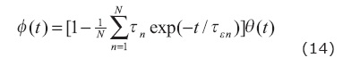
where * denotes the convolution in time, and (t) is the specific creep function. For one dissipation mechanism,

where θ - the Heaviside function, and τ= 1-τ_σ /τ_ε, provided τ_ε>τ_σ. For small t<<τ_ε, it corresponds to the hyperbolic creep function used by Lomnitz (1957).

By taking the time derivative of (2), and substituting the dependence of strain on the particle velocity

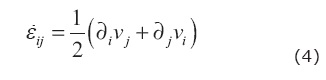
one can get:

where λ and μ- Lame elastic constants, {i=x,z; j=x,z} for two-dimensional viscoelastic media, and {i=x,y,z; j=x,y,z} for three-dimensional viscoelastic media.

By expanding in the convolution the time derivative of (see Robertsson et al., 1994), one can get from (5):

where r_ij - the so-called memory variable:

By taking the time derivative of (7), one can get the equation for the memory variable:

Combining (6) and (8), one can obtain a more convenient form of (6):

Adding Newton's second law

yields the system of equations (8)-(10) for the seismic wave propagation in the viscoelastic media, which governs the stress σ_ij, the particle velocity v_i , and the memory variable r_ij in the area of modeling for the case of one dissipation mechanism.

In the case of τ_σ=τ_ε , the system (8)-(10) becomes the system for elastic media.

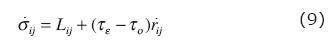
By substituting E_ij= σ_ij-(τ_ε-τ_σ)r_ij one can transform (9) into the equation for elastic media _ij- = L_ij, and obtain from (8):

The equation (11) is similar to equation (1), and can be derived directly from it by defining E_ij = G_ijkl ε_kl. Therefore, the value E has a sense of the elastic part of the stress σ. Thus, the equation (11) governs an effect of viscosity, and it is an equation on only time.

Possibly, we ought to consider two sets of relaxation times: for shear and compressional waves, and modify the equations (8) and (9) by a way following Carcione (1995), for example. But Xu and McMechan (1995) simplified the problem by supposing equal relaxation times for shear and compressional waves. Another way of simplification is to consider cases of multiple dissipation mechanisms which can be transformed to the case of one dissipation mechanism, as below.

For the general case of N dissipation mechanisms which differ only by values of τ_ε, and τ_σ, we should write equations (1) and (2) for each n–th dissipation mechanism as follows:

Values of total σ_ij and ε_ij over N dissipation mechanisms depend on scheme of interactions (interconnections) of the mechanisms: which mechanisms interact as parallel or as sequential, and which groups of mechanisms interact with other groups as parallel or sequential.

Really, the scheme of interactions of mechanisms is not known beforehand, and the problem of modeling does not need such fine developing.

For three simple cases below, it is possible to reduce the system of equations for N mechanisms to the case of one mechanism. They are: 1) N mechanisms interacting sequentialy, 2) N mechanisms interacting in parallel, and 3) two independent groups: one including N₁ mechanisms interacting sequentialy, and the second including N₂ mechanisms interacting in parallel, N₁+ N₂=N. These are general enough cases.

For the case 1), the creep function can be represented as follows (for details see Appendix A):

If introduce the average values of relaxation times:

where R_ij is the average memory variable, which can be found from the following similar equation

For the case 2), the equation (5) becomes as follows:

in which the creep function is (see Appendix A, and Carcione, 1995)

where

For the case 3), the equation (5) is valid for the first group, and the equation (17) is valid for the second group.

Consequently, (if use is done the average memory variable and the average values of relaxation times), one may clearly see that the equations for the considered cases of N mechanisms (15)-(16) are equivalent to equations (6) and (8) for the case of one dissipation mechanism.

From this equivalence, it follows that, for a fixed geometry of the problem, the value of Q depends only on values of , and , and on the source of seismic wave.

Anyway, the solution of equation (11), which is similar to (1), is basic for the case of N mechanisms. Therefore, we will consider the equations for one dissipation mechanism (8) and (9) as the basic equations, and for this case, will calculate the dependence of factor Q on the average relaxation times of the media.

Solution method for the model

The system of equations (8)–(10) is solved by the finite–difference method with using the PML for boundary conditions. The finite–difference scheme has the following form:

where

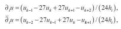
where h_i - the space step in the i–direction, and k- the space mesh index in the i-direction. If an inner boundary of the area coincides with a middle line between the nodes, the average coefficients ¡, _i, and _i for the inner boundary are calculated as follows:

The scheme (19) is written for a fixed grid (k_i= 0.....I; k_j = 0.....J; k_k=0.....K; n = 0, 1, 2, ...), and has the order of approximation O (Δt²,h⁴). It is practically equivalent to the "staggered" scheme used by Virieux (1986), and by Robertsson et al. (1994), but it operates only with integer values of indexes, as classical schemes, what is achieved by appropriate shift of "staggered" indexes.

The equation (19a) can be solved by implicit scheme. It gives:

The necessary stability condition for the scheme (19)-(20) in the 3D case is:

Where

where ƒ - the Ricker wavelet frequency. This condition provides the undamaged form of PP, PS, and SS waves in seismograms. The coefficient 16 is empirical and can be explained by 4-point approximation of space derivatives and 4-slope form of the Ricker wavelet. It should not be less than 4 points at each slope. Other authors suggest different values of the coefficient for schemes of different accuracy: 10 - Virieux (1986), 12 - Moczo et al. (1997), 15-20 - Xu and McMechan (1998).

Above, V_p and V_s are velocities of the compressional and shear waves used in definition of the Lame constants.

In the nodes of the PML absorbing layer, the equations (19b)-(19c) are modified by Collino and Tsogka (2001). Indeed, I apply another formula for absorbing sink (S_a) in the left hand side of the modified equations (19b,c). It forms the implicit (not centered) scheme with the finite-difference time derivative (Sabinin et al., 2003):

where u - the same variable that is in the finite-difference time derivative of the corresponding equation of the system (19).

The parameter d in (22) is calculated by a new formula (k = x, y, z - index of direction):

Advantage of the finite-difference scheme (19)-(23) is its convenience for parallel computations what are easily done with instructions of Open MP.

Estimation of factor Q

For obtaining dependence of the quality factor Q on relaxation times, let us consider a formula by Liu et al. (1976), which is valid under the assumption that τ_ε and τ_σ do not depend on frequency ω=2πƒ at the specified bandwidth:

Taking an integral from this expression over some interval of frequency, one can get the formula

where the constant coefficients a, and b are to be evaluated from a numerical experiment. The formula (24) is derived without the assumption τ<<1 used by Blanch et al. (1995).

From different methods of estimation for factor Q (see, for example, Tonn, 1991), two methods seem as more reliable.

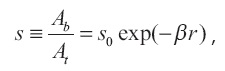
where A_t, A_b - amplitudes of spectra of reflection waves from top and bottom of the target layer in the same ray path, r is a travel distance, and β is an absorption coefficient.

Futterman (1962) defined the quality factor Q as

where

ƒ is frequency, and τ₀ is a travel time. It means that Q>2π.

From the other hand, one can approximate a logarithm of the same spectral ratio by a line function over a proper interval of ƒ by the least squares method:

The art of application of this method consists in proper choice of a window for impulse in the time domain, and a window (interval) for the least squares method in the spectral domain.

For the Ricker wavelet which will be used further, the time window must include all three phases of the impulse up to visible noise at the edges. It is a visible width of impulse at the seismogram.

The spectrum of the Ricker impulse has a shape of a bell, and a logarithm of the spectral ratio has a near line part (see Fig. 1). The spectral window should be chosen inside this line part. It can be made manually. For automatic choice, by observing synthetic seismograms, it was found that a good choice is the window between 0.8 of the peak frequency for the bottom spectrum and the peak frequency for the top spectrum.

The second method used is the Centroid Frequency Shift (FS) method (Quan and Harris, 1993). Here the coefficient r for the formula (26) is calculated by the following formulas:

where s depends on the shape of spectra, for Gaussian spectra s=1 (Quan and Harris, 1993).

The FS method operates with integral values, therefore it is less sensitive to the noise than the SR method, but it is more sensitive to the shape of spectra.

Because of influence of errors on the shape of spectra, it is used the same spectral window for the FS method as for the SR method.

To calculate τ₀ in a multilayered reservoir, a system of non-linear equations can be derived by the ray-tracing method (see Appendix C).

If the target layer is the second from the surface, then the calculations become simpler. Ray paths for this case are presented in Figure 2. One can see that

where indexes 1, and 2 denote the number of layer from above, V is V_p, r₀ is the path from a source to the top of target layer for the impulse reflected from the top, r₁ is the same for the impulse reflected from the bottom, r₂ is the path inside the second layer from the top to the bottom of target layer, and Δt is time between the reflected impulses at the trace.

For reflection data, the receivers are at the surface, therefore τ₀ is twice more than travel time between points x , and x₀.

Using Snell's law, one excludes the velocity V₂ of the target layer from (28):

where p = 0.5ΔtV₁ +, x₀ is the half of the offset, z₁, z₂ are thicknesses of the layers, and θ₁, θ₂ are travel (incidence) angles.

The non-linear equation (30) is solved numerically. The obtained value x is used to calculate the travel time τ₀=2r₂/V₂ of the ray inside the target layer. From (28),

where V₁ is V_p of the upper layer. The value Δt can be calculated by the correlation function between the impulses at the trace.

Difference between Δt and τ₀ is illustrated in Figure 3. The difference increases with offset significantly.

An advantage of the method (30)-(31) is the exclusion of the unknown velocity V₂ from consideration.

As can be also seen from Fig. 2, for more exact estimating the factor Q, one should use the wave reflected from the point x at the top of target layer to calculate spectral amplitude A_t, but not from the point x₀ which is commonly used for this purpose. Knowing value x from (30), one may obtain this wave (or its spectrum) by interpolation from waves (or spectra) of adjacent traces, with taking into account different values of geometrical spreading.

Another possible problem in estimating Q of the target layer is how to exclude from the consideration the coefficients of reflection and refraction at the boundaries of the viscoelastic target layer. It will be the best result in the estimation of Q if the spectral amplitudes will differ only because of viscoelastic attenuation inside the layer. Really, the reflection and refraction at the boundaries of the layer may also act:

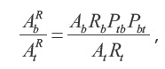
If R and P would depend on f then they influenced on value of Q. However, practice shows that influence of reflection/refraction coefficients on the estimated values of Q is less than difference in estimated values Q caused by different smart choices of the time and spectral windows.

Both methods SR and FS give close values Q but FS insufficiently less.

Numerical simulation

I use the developed numerical model for obtaining the synthetic seismograms of waves reflected from the top and bottom boundaries of a horizontal viscoelastic layer. Then I estimate the factor Q from the seismograms with different τ, and τ_σ, and put these values into the left-hand side of the formula (24) to estimate the values of the coefficients a, b of the formula (24) by least squares method.

The computation of synthetic seismograms by the viscoelastic model was performed at a workstation which gave possibility to parallelize calculations into 24 threats. But it was too slow for a 3D model. For economy, a 2D problem was chosen for the numerical experiment, as follows.

At the earth surface, there was one wave source, and a set of equally spaced (every 100 meters) receivers (the common source point observation system). The area of width 5000 m and depth 2250 m consisted of three homogeneous layers, the target viscoelastic layer was the second, beginning at the depth 1500 m, and had the thickness 400 m. The other layers were considered as elastic, with τ = 0.

The density, and the elastic velocities of compressional and shear waves were as in Table 1.

Seismic wave source of explosion type was the Ricker wavelet in time, its frequency ƒ_r was set to 15, 30, 45, and 60 Hz, duration of the impulse -160, 80, 53.3, and 40 ms correspondingly.

The mesh sizes of the finite-difference grid were h_x=5m, h_z=2.5m, and the time step was 0.2 ms. The PML thickness was equal to 40 nodes. The PML was not mounted at the earth surface where the source was set.

The typical seismogram of v_z obtained for this 2D problem is shown in Figure 4. First two fronts of PP-waves were used for estimating the factor Q. PP waves reflected from the bottom of area (1400-1500 ms), and direct waves reflected from the vertical sides of area are not visible. It means a good effectiveness of applied modification of PML absorbing boundaries.

For comparison, the 3D problem was computed in the variant of ƒ_r = 30 Hz, τ= 0.7, and τ_σ= 0.625ms. The 3D area had and additionally y-direction with thickness 2000 m. The receivers were spaced in the middle line. For saving time of computation, a rough grid was used: h_x=h_y=20m, and the time step 0.4ms.

The seismogram of v_z obtained for the 3D problem is shown in the Figure 5. Visible distortions are caused by the roughness of grid The Figure 5 corresponds to the variant of Figure 4. Values of factor Q calculated for seismograms of Figures 4, and 5 are practically the same, and are equal to 14.8.

The comparison is good enough to decide to apply more economical 2D model in the numerical experiment.

Numerical results

Factor Q was calculated with the SR method for all offsets and did not show any stable or significant dependence on the offset. Existing errors were caused by small distortions of waves by interference with waves reflected from the sides of area, and by errors in setting the time windows.

Difficulty in calculation of the factor Q is that the linear part of logarithm of spectral ratio which one can see in Figure 1 is not clearly present for extreme values of relaxation times. For example, it is a curve for large values τ_σ. Therefore, this gave unreliable values of Q sometimes.

The results of calculation of factor Q in a wide range near normal incidence are presented in Tables 2-5 (3-4) for the source frequencies of ƒ_r =15, 30, 45, 60 Hz respectively.

As equations (8), (9) depend on τ and τ_σ, so the values Q in the Tables 2-5 (3-4) are presented depending on these parameters. Also, the results depend on the frequency of the source significantly.

It was found that equation (24) does not match satisfactory to Tables 2-5 (3-4). Instead, the following similar equation was derived for this:

where d depends on Q by formula (25), x=τ^α , y=[3/(ƒ_rτ_σ)]^β. Values α=0.7, and β=1.2 represent a near optimal choice.

The obtained coefficients A, B, and C of (32) are presented in Table 6 with values of relative estimation error by (32).

For practical use, one can apply Tables 2-5 (3-4), or equation (32), or derive an own approximation formula.

Discussion

Some authors (Blanch et al., 1995; Xu and McMechan, 1998) guess that the constant value Q over some interval of spectral frequency, which one can usually see, is equal to a near constant value Q on an average graphic consisting of the separate theoretical graphics Q (as by Liu et al., 1976) for N>1 dissipation mechanisms with different relaxation times. As one can see from (25), this method of obtaining constant Q fails in the case of one dissipation mechanism. Contrary, the experimental formula (32) does not depend on the number of dissipation mechanisms.

Although the formulas (25) - (27) of methods for estimating factor Q are simple, they have several sources for errors. At first, it is a nonlinear form of the "line" part of the logarithm of spectral ratio which can be clearly seen in field data. It is necessary smoothing seismograms with noise, and developing new methods of Q-estimation for synthetic seismograms obtained at large τ_σ.

Second, insignificantly different sizes and positions of time windows can give significantly different spectra what is caused by increased role of noise at the edges of impulses. Suitable automatic algorithms for generating the time windows are needed.

Third, a correct estimation of the travel time is needed as one can see from Figure 3.

Finally, a good estimation for the usually unknown impulses reflected from the top of target layer in the point x of Fig.2 is necessary.

Errors from these four sources can give significantly incorrect values Q, up to 50% and more.

As known, PML absorbing boundary does not exclude completely reflections from the boundaries of area for finite-difference problems. The modification of PML presented here decreases the reflections in comparison with classical PML by Collino and Tsogka (2001) due to lucky choice of exponent functions for approximation (23).

Errors of the approximated formula (32) for dependence Q on relaxation times are in agreement with errors of estimating Q. For example, if it is excluded the first and ultimate columns from Table 2, then the error of estimation by (32) becomes twice less.

Conclusion

A numerical 3D model for seismic wave propagation in viscoelastic media is developed, which differs from the previous (Robertsson et al. 1994) by modification of the finite-difference scheme, and by including the improved variant of PML absorbing boundary.

It is shown that the numerical model for one dissipation mechanism can be directly applied to three simple schemes of interaction of N dissipation mechanisms by using average relaxation times.

The synthetic seismograms are obtained for 3D, and 2D variants of a reservoir which show close values of factor Q in the viscoelastic layer.

The methodology of estimation of factor Q for surface reflection data is developed which differs from previous by more exact calculation of travel times for reflected waves, and by manual choice of spectral windows. The viscoelastic model and the method of Q-estimation are applied to obtaining experimental dependences of factor Q on relaxation times. The approximate formula is suggested for such dependence.

Blanch J.O, Robertsson J.O.A., Symes W.W.,1995, Modeling of constant Q: Methodology and algorithm for an efficient and optimally inexpensive viscoelastic technique, Geophysics, 60, 1, p.176-184.         [ Links ]

Carcione J.M., 1993, Seismic modeling in viscoelastic media, Geophysics, 58, 1, p.110-120.         [ Links ]

Carcione J.M., 1995, Constitutive model and wave equations for linear, viscoelastic, anisotropic media, Geophysics, 60, 2, p.537-548.         [ Links ]

Carcione J.M., Kosloff D., Kosloff R., 1988, Wave propagation in a linear viscoelastic medium, Geophysical Journal, 95, p.597-611.         [ Links ]

Collino F., Tsogka C., 2001, Application of the PML Absorbing Layer Model to the Linear Elastodynamic Problem in Anisotropic Heterogeneous Media, Geophysics, 66, 1, 294-307.         [ Links ]

Dasgupta R., Clark R.A., 1998, Estimation of Q from surface seismic reflection data. Geophysics, 63, 2120-2128.         [ Links ]

Emmerich H., 1992, PSV-wave propagation in a medium with local heterogeneities: a hybrid formulation and its application, Geophys. J. Int., 109, 54 - 64.         [ Links ]

Futterman W.I., 1962, Dispersive body waves. J. Geophys. Res, 67, 5279-5291.         [ Links ]

Knopoff L., 1964, Q. Revs. Geophys, 2, 625-660.         [ Links ]

Komatitsch D., Tromp J., 2002, Spectral-element simulations of global seismic wave propagation- I. Validation. Geophys. J. Int., 149, p.390- 412.         [ Links ]

Liu H.-P., Anderson D.L., Kanamori H., 1976, Velocity dispersion due to anelasticity; implications for seismology and mantle composition, Geophys. J. R. Astr. Soc., 47, 41-58.         [ Links ]

Lomnitz C., 1957, Linear dissipation in solids. J. Appl. Phys., 28, 201-205.         [ Links ]

Mikhailenko B., Mikhailov A., Reshetova G., 2003, Spectral Laguerre method for viscoelastic seismic modeling. Mathematical and Numerical Aspects of Wave Propagation WAVES 2003, Springer-Verlag, p.891-896.         [ Links ]

Moczo P., Bystricky E., Kristek J., Carcione J.M., Bouchon M., 1997, Hybrid modeling of P-SV seismic motion at inhomogeneous viscoelastic topographic structures, Bulletin of the Seismological Society of America, 87,5, p.1305-1323.         [ Links ]

Quan Y., Harris J.M., 1993, Seismic attenuation tomography based on centroid frequency shift, Exp. Abs., 63-rd Ann. Internat. SEG Mtg., Washington, Paper BG2.3.         [ Links ]

Robertsson J.O.A., Blanch J.O., Symes W.W., 1994, Viscoelastic finite-difference modeling. Geophysics, 59, 9, p.1444 - 1456.         [ Links ]

Sabinin V., Chichinina T., Ronquillo Jarillo G., 2003, Numerical model of seismic wave propagation in viscoelastic media. Mathematical and Numerical Aspects of Wave Propagation WAVES 2003, Springer-Verlag, p.922-927.         [ Links ]

Tonn R., 1991, The determination of the seismic quality factor Q from VSP data: a comparison of different computational methods, Geophysical Prospecting, 39, 1-37.         [ Links ]

Virieux J., 1986, P-SV wave propagation in heterogeneous media: Velocity-stress finite-difference method. Geophysics, 51, 4, p.889- 901.         [ Links ]

Xu T., McMechan G.A., 1995, Composite memory variables for viscoelastic synthetic seismograms. Geophys. J. Int, 121, p.634 -639.         [ Links ]

Xu T., McMechan G.A., 1998, Efficient 3-D viscoelastic modeling with application to near-surface data. Geophysics, 63, 2, p.601 - 612.         [ Links ]