<?xml version="1.0" encoding="ISO-8859-1"?><article xmlns:mml="http://www.w3.org/1998/Math/MathML" xmlns:xlink="http://www.w3.org/1999/xlink" xmlns:xsi="http://www.w3.org/2001/XMLSchema-instance">
<front>
<journal-meta>
<journal-id>0187-6236</journal-id>
<journal-title><![CDATA[Atmósfera]]></journal-title>
<abbrev-journal-title><![CDATA[Atmósfera]]></abbrev-journal-title>
<issn>0187-6236</issn>
<publisher>
<publisher-name><![CDATA[Universidad Nacional Autónoma de México, Instituto de Ciencias de la Atmósfera y Cambio Climático]]></publisher-name>
</publisher>
</journal-meta>
<article-meta>
<article-id>S0187-62362008000400006</article-id>
<title-group>
<article-title xml:lang="en"><![CDATA[Influence of synoptic scale in the generation of extremely cold days in Europe]]></article-title>
</title-group>
<contrib-group>
<contrib contrib-type="author">
<name>
<surname><![CDATA[CONY]]></surname>
<given-names><![CDATA[M]]></given-names>
</name>
<xref ref-type="aff" rid="A01"/>
</contrib>
<contrib contrib-type="author">
<name>
<surname><![CDATA[HERNÁNDEZ]]></surname>
<given-names><![CDATA[E]]></given-names>
</name>
<xref ref-type="aff" rid="A01"/>
</contrib>
<contrib contrib-type="author">
<name>
<surname><![CDATA[DEL TESO]]></surname>
<given-names><![CDATA[T]]></given-names>
</name>
<xref ref-type="aff" rid="A01"/>
</contrib>
</contrib-group>
<aff id="A01">
<institution><![CDATA[,Universidad Complutense de Madrid Facultad de Ciencias Físicas Departamento de Física de la Tierra II]]></institution>
<addr-line><![CDATA[ ]]></addr-line>
<country>España</country>
</aff>
<pub-date pub-type="pub">
<day>00</day>
<month>10</month>
<year>2008</year>
</pub-date>
<pub-date pub-type="epub">
<day>00</day>
<month>10</month>
<year>2008</year>
</pub-date>
<volume>21</volume>
<numero>4</numero>
<fpage>389</fpage>
<lpage>401</lpage>
<copyright-statement/>
<copyright-year/>
<self-uri xlink:href="http://www.scielo.org.mx/scielo.php?script=sci_arttext&amp;pid=S0187-62362008000400006&amp;lng=en&amp;nrm=iso"></self-uri><self-uri xlink:href="http://www.scielo.org.mx/scielo.php?script=sci_abstract&amp;pid=S0187-62362008000400006&amp;lng=en&amp;nrm=iso"></self-uri><self-uri xlink:href="http://www.scielo.org.mx/scielo.php?script=sci_pdf&amp;pid=S0187-62362008000400006&amp;lng=en&amp;nrm=iso"></self-uri><abstract abstract-type="short" xml:lang="es"><p><![CDATA[Una base de datos homogéneos de temperaturas mínimas de 135 observatorios distribuidos en Europa ha sido analizada con el objetivo de estimar las variaciones de tendencias e identificar las principales situaciones sinópticas que contribuyen en un día de frío extremo (DFE). Se ha considerado un Día de Frío Extremo (DFE) definido por el percentil 5% de la serie de temperatura mínima diaria de cada observatorio; valores que tiene efectos sobre la salud. Para este análisis se utiliza el periodo de 1 de enero de 1955 hasta el 31 de diciembre de 1998; período que presenta el mayor número de estaciones de medidas con series completas. La conexión entre los DFE con la circulación general de la atmósfera, está basada en un análisis detallado obteniendo un coeficiente de eficacia para cada patrón sinóptico. Para simplificar la información obtenida, se aplica un análisis de componentes principales rotadas (RPC) y se obtienen los patrones sinópticos con mayor contribución a los DFE. Al mismo tiempo se ha hecho un análisis de tendencia en cada uno de los patrones sinópticos y también un estudio comparativo entre los diferentes DFE de las situaciones sinópticas.]]></p></abstract>
<abstract abstract-type="short" xml:lang="en"><p><![CDATA[A homogenized database of minimum temperatures from 135 observatories distributed around Europe was analyzed in order to estimate trends and to determine the main synoptic weather patterns that contribute to an extremely cold day (ECD). An ECD is defined as a day whose minimum temperature is within the lowest 5th centile of the daily temperature series for each observatory; these values represent temperatures below which public health concerns may be expected. The period from 1 January 1955 to 31 December 1998 was chosen for this analysis because it represents the period for which the greatest number of measuring stations with complete time series was available. The relationship between the occurrence of an ECD and the general circulation of the atmosphere was based on a statistical analysis in which a coefficient of effectiveness for each synoptic pattern was obtained. In order to simplify the manipulation of the data, a rotated principal components (RPC) analysis was applied and the synoptic patterns with the greatest contribution to the ECD were obtained. Trends for each synoptic pattern were studied in order to examine the relationship among the ECD.]]></p></abstract>
<kwd-group>
<kwd lng="en"><![CDATA[Extremely cold days]]></kwd>
<kwd lng="en"><![CDATA[GWL patterns]]></kwd>
<kwd lng="en"><![CDATA[ECD over Europe]]></kwd>
</kwd-group>
</article-meta>
</front><body><![CDATA[ <p align="center"><font face="verdana" size="4"><b>Influence of synoptic scale in the generation of extremely cold days in Europe</b></font></p>     <p align="center"><font face="verdana" size="2">&nbsp;</font></p>     <p align="center"><font face="verdana" size="2"><b>M. CONY, E. HERN&Aacute;NDEZ and T. DEL TESO</b>    <br>     <i>Departamento de F&iacute;sica de la Tierra II, Facultad de Ciencias F&iacute;sicas,</i>    <br>   <i>Universidad Complutense de Madrid, Espa&ntilde;a </i>    <br>   Corresponding author: M. Cony; e&#150;mail: <a href="mailto:macony@fis.ucm.es" target="_blank">macony@fis.ucm.es</a></font></p>     <p align="center"><font face="verdana" size="2">&nbsp;</font></p>     <p align="center"><font face="verdana" size="2">Received February 7, 2008; accepted June 11, 2008 </font></p>     <p align="justify"><font face="verdana" size="2">&nbsp;</font></p>     <p align="justify"><font face="verdana" size="2"><b>RESUMEN</b></font></p>     ]]></body>
<body><![CDATA[<p align="justify"><font face="verdana" size="2">Una base de datos homog&eacute;neos de temperaturas m&iacute;nimas de 135 observatorios distribuidos en Europa ha sido analizada con el objetivo de estimar las variaciones de tendencias e identificar las principales situaciones sin&oacute;pticas que contribuyen en un d&iacute;a de fr&iacute;o extremo (DFE). Se ha considerado un D&iacute;a de Fr&iacute;o Extremo (DFE) definido por el percentil 5% de la serie de temperatura m&iacute;nima diaria de cada observatorio; valores que tiene efectos sobre la salud. Para este an&aacute;lisis se utiliza el periodo de 1 de enero de 1955 hasta el 31 de diciembre de 1998; per&iacute;odo que presenta el mayor n&uacute;mero de estaciones de medidas con series completas. La conexi&oacute;n entre los DFE con la circulaci&oacute;n general de la atm&oacute;sfera, est&aacute; basada en un an&aacute;lisis detallado obteniendo un coeficiente de eficacia para cada patr&oacute;n sin&oacute;ptico. Para simplificar la informaci&oacute;n obtenida, se aplica un an&aacute;lisis de componentes principales rotadas (RPC) y se obtienen los patrones sin&oacute;pticos con mayor contribuci&oacute;n a los DFE. Al mismo tiempo se ha hecho un an&aacute;lisis de tendencia en cada uno de los patrones sin&oacute;pticos y tambi&eacute;n un estudio comparativo entre los diferentes DFE de las situaciones sin&oacute;pticas.</font></p>     <p align="justify"><font face="verdana" size="2">&nbsp;</font></p>     <p align="justify"><font face="verdana" size="2"><b>ABSTRACT</b></font></p>     <p align="justify"><font face="verdana" size="2">A homogenized database of minimum temperatures from 135 observatories distributed around Europe was analyzed in order to estimate trends and to determine the main synoptic weather patterns that contribute to an extremely cold day (ECD). An ECD is defined as a day whose minimum temperature is within the lowest 5th centile of the daily temperature series for each observatory; these values represent temperatures below which public health concerns may be expected. The period from 1 January 1955 to 31 December 1998 was chosen for this analysis because it represents the period for which the greatest number of measuring stations with complete time series was available. The relationship between the occurrence of an ECD and the general circulation of the atmosphere was based on a statistical analysis in which a coefficient of effectiveness for each synoptic pattern was obtained. In order to simplify the manipulation of the data, a rotated principal components (RPC) analysis was applied and the synoptic patterns with the greatest contribution to the ECD were obtained. Trends for each synoptic pattern were studied in order to examine the relationship among the ECD.</font></p>     <p align="justify"><font face="verdana" size="2"><b>Keywords:</b> Extremely cold days, GWL patterns, ECD over Europe.</font></p>     <p align="justify"><font face="verdana" size="2">&nbsp;</font></p>     <p align="justify"><font face="verdana" size="2"><b>1.</b>&nbsp;<b>Introduction</b></font></p>     <p align="justify"><font face="verdana" size="2">The increase in the global mean temperature during the twentieth century, in particular over the last 30 years, has provided a strong incentive for investigations of climate change. The average global temperature has increased by approximately 0.6&deg; C between the end of the nineteenth century and the present day (IPCC, 2001). For this time interval, two periods of strong global warming have been identified, firstly between 1910 and the early 1940s, and secondly between the mid 1970s and the present day (Jones <i>et al., </i>1999; Karl <i>et al, </i>2000). It has been confirmed that in Europe the majority of the increases of temperature coincide with periods when global temperatures also increased (Klein Tank <i>et al., </i>2002). Analyses of temperature records show that warming does not happen homogeneously but is instead concentrated around certain specific regions (Easterling <i>et al., </i>1997), thus requiring research that is focused on the study of temperatures within these regions.</font></p>     <p align="justify"><font face="verdana" size="2">Heat or cold waves are characterized by the occurrence of a sequence of days with high or low values of temperature. These waves have significant impacts in terms of their socioeconomic effects on health, agriculture, forest fires, and the production and consumption of energy (SIAM, 2002; Garc&iacute;a&#150;Herrera <i>et al., </i>2005; Pereira et al., 2005; Trigo <i>et al., </i>2005). Observations from some European capitals show a direct and proportional relationship between extreme temperatures and their impacts on public health (D&iacute;az <i>et al., </i>2002). Both maximum and minimum extremes in temperature are associated with impacts on public health, although the relation between minimum temperatures in winter and mortality is not as noticeable as the equivalent high&#150;temperature relationship during summer months. It is clear that the effect of the cold on mortality depends on the time of exposure to these temperatures and, in addition, minimum extreme temperatures occur in general in the hours before dawn, when people are usually indoors and are thus protected from their effects. However, it is possible to find a relationship between low temperatures and the occurrence and intensification of breathing problems (Hajat and Haines, 2002). D&iacute;az <i>et al. </i>(2004) verified that the effects of cold waves do not generally cause sudden death, but may instead lead to a fatality several days later, unlike the effects of the summer temperature maxima.</font></p>     <p align="justify"><font face="verdana" size="2">The aim of the present study is to determine the influence of synoptic patterns that cause extreme daily minimum temperatures. To do so, we will select the series of daily minimum temperatures in 34 European countries and the main synoptic patterns that occur in Europe, in the near&#150;surface region and at different altitudes, associated with particular sequences of extremely cold days.</font></p>     ]]></body>
<body><![CDATA[<p align="justify"><font face="verdana" size="2">The present study is structured as follows: Section 2 contains a discussion of the trends analysis used in this study. In Section 3, the data used and the methodology applied to the synoptic weather patterns are described, as well as the method of identification of those synoptic patterns that have the greatest impact on the occurrence of extremely cold days (ECD). This section also contains an analysis of the trends of the synoptic patterns for the period of study. Section 4 concludes.</font></p>     <p align="justify"><font face="verdana" size="2">&nbsp;</font></p>     <p align="justify"><font face="verdana" size="2"><b>2.</b>&nbsp;<b>Temporal analysis</b></font></p>     <p align="justify"><font face="verdana" size="2">In this section, the temporal analysis technique, based on the investigation of trends leading to the occurrence of ECD is explained. Firstly, the characterization and methodology applied to the series of daily minimum temperatures is described. Next, an ECD is defined. Finally, the processes and results of trends based on the annual frequency of ECD are discussed, as well as the factors that contribute to the increase or decrease in extreme minimum temperatures.</font></p>     <p align="justify"><font face="verdana" size="2">&nbsp;</font></p>     <p align="justify"><font face="verdana" size="2"><i>2.1 Minimum temperature series</i></font></p>     <p align="justify"><font face="verdana" size="2">
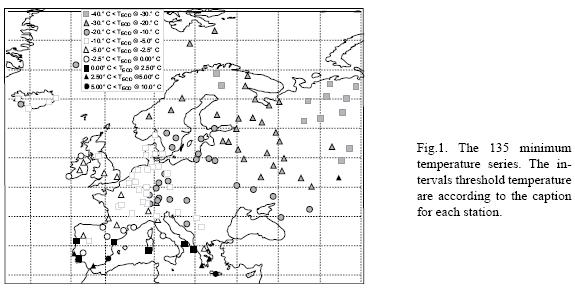
The series of minimum daily temperatures used here were obtained from the ECA Dataset (Klein Tank <i>et al., </i>2002), which is available on&#150;line for the 44 years from 1 January 1955 to 31 December 1998. This data set was chosen because it possesses the greatest number of complete time series of temperatures. Station selection was based on the need to cover as much European territory as possible. In total, 135 time series of distributed minimum temperatures in 34 countries were selected (<a href="#f1">Fig 1</a>).</font></p>     <p align="center"><font face="verdana" size="2"><a name="f1"></a></font></p>     <p align="center"><font face="verdana" size="2"><img src="/img/revistas/atm/v21n4/a6f1.jpg" alt=""></font></p>     <p align="justify"><font face="verdana" size="2">The time series of minimum temperature (<i>Tmin</i>) were selected and subjected to a homogenization process in order to eliminate discontinuities (Easterling <i>et al., </i>1992; Della&#150;Marta et al., 2005). In this case, the techniques of homogenization applied in this study are similar to those developed by Peterson and Easterling (1994), and used by Prieto <i>et al. </i>(2002). The technique consists, firstly, on the construction of an homogenous reference series from nearby stations that show a similar variability in the observed parameters. In the same way as Peterson and Easterling (1994) it has been decided to take the five nearest stations that showed the greatest correlation with the original series. We evaluated the use of five different methods of spatial interpolation: multiple discrimination analysis (Miller, 1962), multiple linear regression, standardized anomaly, weighted average, and an average of the four previous methods. Of these, the weighted average method produced the best results. Using this method, series of annual average temperatures for the 135 stations were created and were used as a reference for the rest of the analyses. In all the time series, a method of 'search and detection' for discontinuities was applied, the technique used being similar to that of Easterling and Peterson (1995).</font></p>     ]]></body>
<body><![CDATA[<p align="justify"><font face="verdana" size="2">&nbsp;</font></p>     <p align="justify"><font face="verdana" size="2"><i>2.2 Extremely cold days</i></font></p>     <p align="justify"><font face="verdana" size="2">In a previous work on extreme temperatures, threshold temperatures have been used to identify days of extreme cold or heat. Some studies define an extreme in temperature on the basis of the impacts that they have on the environment, but there are other purely statistical definitions. In this case, the 1st, 5th or 10th percentile of the minimum temperature series, and the 99th, 95th or 90th centile in the case of maximum temperatures series, are used (DeGaetano, 1996).</font></p>     <p align="justify"><font face="verdana" size="2">In our analysis, we used the 5th centile of the series of minimum temperatures. This was computed for each of the 135 time series of temperatures selected from November to March. Therefore, an ECD is defined as a day on which the minimum temperature lies within the 5 percentile of the distribution of daily minimum temperature series. This threshold in the series of minimum temperatures agrees with studies in Spain that demonstrate it as having the most significant impact on public health (D&iacute;az <i>et al., </i>2003).</font></p>     <p align="justify"><font face="verdana" size="2"><a href="#f1">Figure 1</a> shows the different thresholds in temperature for each station from measurements distributed within the 34 European countries. The distribution of thresholds in minimum temperatures varies between 6.1&deg; C at Heraklion (Greece, Lat. 35.33&deg;/ Lon. 25.18&deg;) to &#150;39.1&deg; C at Hoseda Hard (Russia, Lat. 67.08&deg;/Lon. 59.38&deg;). It is evident that the temperature thresholds are lower at higher latitudes and altitudes, for instance, at Zugspitze (Germany, Lat. 47.25&deg;/Lon. 10.59&deg;, altitude 2960 m) the threshold is &#150;21.4&deg; C.</font></p>     <p align="justify"><font face="verdana" size="2">However, the selection of temperature thresholds is not critical to the determination of the frequency of ECD, when the interannual variability in temperature is taken into account. The series of annual frequencies of ECD does depend on the temperature threshold selected, but it is much more sensitive to the interannual variability in temperature. In order to verify this, the series of annual frequencies of ECD, was calculated by considering a difference of 1&deg; C in selected threshold values. For most stations, this yields a variation in threshold of from 2 to 8 percent of the original value. Comparison of the series with the new thresholds and the series obtained using the original thresholds shows an average correlation coefficient of around 0.93 (at the level of 99.9%), with a maximum of a 0.98 and minimum of 0.82. It therefore follows that most of the variability of the ECD frequency series does not depend on the threshold selected and thus, the threshold used here will provide information relating to the interannual variability of ECD.</font></p>     <p align="justify"><font face="verdana" size="2">&nbsp;</font></p>     <p align="justify"><font face="verdana" size="2"><i>2.3 ECD trend over Europe</i></font></p>     <p align="justify"><font face="verdana" size="2">In this analysis, the objective was to verify the trends in the annual frequency of ECD that occurred throughout the whole period of study in the 135 series of minimum temperatures in Europe.</font></p>     <p align="justify"><font face="verdana" size="2">The technique that is used most commonly for calculating meteorological variable trends is linear regression. However, this method cannot be used to calculate extreme temperature trends because the deviations in the observed data do not generally follow normal distributions. Moreover, linear regression is affected by values at the extremes of the series, especially for shorter time series, and this can lead to significant errors. Consequently, it is necessary to use another technique that provides estimations of the trends but avoids this type of error. An alternative method for analyzing trends was developed by Karl and Williams (1987) and later applied in the calculation of extreme frequency trends by DeGaetano (1996). Using this technique, we can obtain reasonable estimates of the trends of annual frequencies that would not be possible with traditional techniques. In order to calculate the significant trends (p), it has been applied a Monte Carlo test. By carrying out this test, 5000 random series disordering the original ones were obtained and the statistical <i>t </i>was calculated for each of them. The trends' significance value was then obtained as the percentage of simulations whose statistical <i>t </i>exceeded the original one.</font></p>     ]]></body>
<body><![CDATA[<p align="justify"><font face="verdana" size="2">This method of tendencies was applied to the 135 annual series of ECD frequency. The results are shown in <a href="#f2">Figure 2</a>, where statistically significant trends at the levels of 99%, 95% and 90% are shown. In all stations, the trends were negative, but in 64.4% of the stations, the measurements showed significantly high trends (p &lt; 0.10). The highest decreases were detected in Mediterranean and Central European observatories.</font></p>     <p align="center"><font face="verdana" size="2"><a name="f2"></a></font></p>     <p align="center"><font face="verdana" size="2"><img src="/img/revistas/atm/v21n4/a6f2.jpg" alt=""></font></p>     <p align="justify"><font face="verdana" size="2">The temperature follows a Gaussian distribution, the variations in the extremes being due mainly to changes in the mean or standard deviation. For this reason, it is important to know the temporal evolution, the average, and the variance of the series of temperature in order to know which of these two factors, minimum average temperature and standard deviation, has a greater influence in the increase or decrease of ECD.</font></p>     <p align="justify"><font face="verdana" size="2"><a href="/img/revistas/atm/v21n4/a6f3.jpg" target="_blank">Figure 3a</a> shows the analysis of trends in the minimum average temperature from November to March for those trends that are positive. An increase may be observed in the majority of the stations. Seventy&#150;three percent of the stations present significant highest positive trends (p &lt; 0.10). It may be observed that stations that show trends in the minimum average temperature do not correspond with stations that present significant trends in the annual frequency of ECD. Therefore, this is an important factor in the decrease of annual occurrence of ECD, because the trends analysis estimates increases between 0.5 and 2.0&deg; C in the minimum temperature. In terms of the standard deviation, the analysis of trends shows that 53.3% of stations with significant measures show negative trends. These results are shown in <a href="/img/revistas/atm/v21n4/a6f3.jpg" target="_blank">Figure 3b</a>. In this case, it may be seen that standard deviation is not an important factor for the decrease of the annual frequency of ECD.</font></p>     <p align="justify"><font face="verdana" size="2">&nbsp;</font></p>     <p align="justify"><font face="verdana" size="2"><b>3. Synoptic scale</b></font></p>     <p align="justify"><font face="verdana" size="2">This section describes the synoptic patterns that have the greatest influence on the generation of extremes of temperature. In Section 3.1, the data obtained from synoptic patterns is described and the reasons for using these weather data are explained. In Section 3.2, the processes used to connect the synoptic patterns and the ECD are described. Finally, in Section 3.3, a method is applied that considers the effect of the synoptic patterns that have the greatest influence on ECD generation, as well as the characterization of each pattern. An analysis of the trends in the synoptic patterns is also described and discussed.</font></p>     <p align="justify"><font face="verdana" size="2">&nbsp;</font></p>     <p align="justify"><font face="verdana" size="2"><i>3.1 The Grosswetterlagen catalogue&#150;GWL</i></font></p>     ]]></body>
<body><![CDATA[<p align="justify"><font face="verdana" size="2">The Grosswetterlagen catalogue (Hess and Brezowsky, 1977; Gerstengarbe and Werner, 1993; Gerstengarbe <i>et al., </i>1999) from 1901 to 1998, inclusive, was used to analyze the statistical relationships between the ECD and the atmospheric synoptic patterns. The classification recognises three groups of circulations types (zonal, half&#150;meridional and meridional), which are divided into ten major types (Grosswettertypen, GWT) and 29 subtypes (Grosswetterlagen, GWL; <a href="/img/revistas/atm/v21n4/a6t1.jpg" target="_blank">Table I</a>).</font></p>     <p align="justify"><font face="verdana" size="2">One of the advantages in using this classification is that it considers the main synoptic patterns that occur in European climates. Fink <i>et al. </i>(2004) used the classification of Hess and Brezowsky for a study of heat waves in 2003 and Domonkos <i>et al. </i>(2003) used it in an analysis of extremes of temperature at eleven stations in central Europe.</font></p>     <p align="justify"><font face="verdana" size="2">&nbsp;</font></p>     <p align="justify"><font face="verdana" size="2"><i>3.2 Connections between ECD and GWL</i></font></p>     <p align="justify"><font face="verdana" size="2">The relationship between an ECD and a synoptic pattern GWL was investigated using statistical tests relating the frequencies of synoptic patterns for those days when an ECD occurred. Once the ECD from each observatory had been identified, a daily classification of the synoptic patterns during these extreme days was obtained.</font></p>     <p align="justify"><font face="verdana" size="2">Using the relationship between the partial relative frequencies (<i>F<sub>%ECD</sub></i>) and total relative frequency (<i>F<sub>%</sub> </i>) of the synoptic patterns and the ECD that occurred during the period of study (November&#150;March), a statistical coefficient was obtained to show the occurrence of a certain synoptic pattern GWL at a certain station. An effectiveness coefficient (EC) may be defined as:
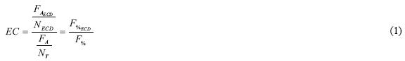
</font></p>     <p align="center"><font face="verdana" size="2"><img src="/img/revistas/atm/v21n4/a6s1.jpg" alt=""></font></p>     <p align="justify"><font face="verdana" size="2">where <i>F<sub>AECD</sub> </i>is the frequency of the synoptic patterns during an ECD, <i>N<sub>ECD</sub> </i>is the number of ECD occurring during the period of study for each observatory, <i>F<sub>A</sub> </i>is the total frequency of synoptic patterns occurring in the months November&#150;March for the whole period, and <i>N<sub>T</sub> </i>is the total number of days (Nov&#150;Mar) throughout all 44 years.</font></p>     <p align="justify"><font face="verdana" size="2">The EC obtained from Eq. (1) may be used to investigate the connection between a GWL pattern and the occurrence of an ECD. A matrix of data is obtained that demonstrates the presence of synoptic patterns. An EC greater than 1 indicates that a certain synoptic pattern has occurred more frequently in a station during an ECD than another one, while an EC less than 1 indicates that the synoptic pattern has occurred less frequently.</font></p>     <p align="justify"><font face="verdana" size="2">&nbsp;</font></p>     ]]></body>
<body><![CDATA[<p align="justify"><font face="verdana" size="2"><i>3.3 Synoptic patterns GWL analysis</i></font></p>     <p align="justify"><font face="verdana" size="2">In order to relate synoptic patterns (GWL) to the occurrence of ECD, a rotated principal components analysis (RPC) was used (White <i>et al., </i>1991), which took into account the EC obtained for every GWL pattern and every observatory under consideration. An RPC analysis considers that all the information of the different series is contained in its variance, and it is for this reason that its matrix&#150;covariance is calculated. In this study, we used the Varimax method, which is commonly used in climatology (Richman, 1986; Stone, 1989; White <i>et al., </i>1991), and to select the number of components to rotate, we used Kaiser's (1958) criterion, which only uses those components with an eigenvalue greater than 1.</font></p>     <p align="justify"><font face="verdana" size="2">To determine the influence of the synoptic patterns in an ECD, in the RPC analysis, we took the first three orthogonal functions (EOF), which explain 68.8% of the accumulated variance. These EOF are represented by a series that comprises a number of coefficients, or weights, that assign to each original series the relative value of this component. By reconstructing the series of these coefficients of EOF it was possible to select the synoptic patterns that have the greatest influence on the generation of an ECD.</font></p>     <p align="justify"><font face="verdana" size="2"><a href="#t2">Table II</a> shows the synoptic patterns through the reconstruction of the series of the coefficients for the first three EOF. It may be observed that patterns of GWL are equal in the three EOF, differing only in the value of the coefficient (in brackets). These five synoptic patterns are therefore the ones that contribute most to the occurrence of an ECD.
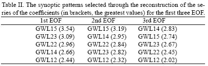
</font></p>     <p align="center"><font face="verdana" size="2"><a name="t2"></a></font></p>     <p align="center"><font face="verdana" size="2"><img src="/img/revistas/atm/v21n4/a6t2.jpg" alt=""></font></p>     <p align="justify"><font face="verdana" size="2"><a href="/img/revistas/atm/v21n4/a6f4.jpg" target="_blank">Figure 4</a> shows maps of anomalies in sea level pressure (SLP) for the emphasized synoptic patterns and similar characteristics are observed among them (<a href="/img/revistas/atm/v21n4/a6f4.jpg" target="_blank">Fig. 4a to e</a>). These characteristics are some types of weak anticyclone in the Atlantic Ocean and European north, successive losses in central and Western Europe, northerly winds, barometric marsh situations in the Mediterranean area (GWL14), and lows in Lithuania and Estonia which introduces cold air towards the center of Europe.</font></p>     <p align="justify"><font face="verdana" size="2">After the greater synoptic patterns that contribute to the occurrence of ECD had been identified, a trends analysis was carried out to verify the behavior of these situations, by taking into account the results obtained in the analysis of the annual frequency of ECD. The methodology used to calculate the trends analysis was the same as that applied in the analysis of trends of ECD. <a href="#t3">Table III</a> shows the results of the trends analysis of the synoptic patterns with negative and significant values in all cases (p &lt; 0.10). In our study, an average decrease in the absolute frequency of the synoptic situations that influence an ECD of &#150;0.10/year was determined.</font></p>     <p align="center"><font face="verdana" size="2"><a name="t3"></a></font></p>     <p align="center"><font face="verdana" size="2"><img src="/img/revistas/atm/v21n4/a6t3.jpg" alt=""></font></p>     ]]></body>
<body><![CDATA[<p align="justify"><font face="verdana" size="2">&nbsp;</font></p>     <p align="justify"><font face="verdana" size="2"><b>4. Discussion and conclusions</b></font></p>     <p align="justify"><font face="verdana" size="2">In this section, the main results obtained in our study are summarized. One hundred and thirty&#150;five complete and homogenous series of distributed daily minimum temperatures in 34 European countries were considered from 1 January 1955 to 31 December 1998.</font></p>     <p align="justify"><font face="verdana" size="2">A methodology is developed in order to analyze trends in the annual frequency of extremely cold days over Europe. The results obtained showed significant negative trends (p &lt; 0.10) at 64.4% of the observatories located in the central and Mediterranean region. In this analysis, temporal evolution of the average minimum temperature and standard deviation were calculated. The results showed significant positive trends (p &lt; 0.10) in the average minimum temperature (73.3% of the measuring stations) and significant negative trends in the standard deviation (53.3% of the measuring stations). It is verified that one of the factors in the decrease of ECD in Europe is the change in the minimum temperature average, which in fact, has increased significantly. The trend analysis estimate an increase of 0.5 to 2.0&deg; C in the average minimum temperature of Europe mainly in the western regions.</font></p>     <p align="justify"><font face="verdana" size="2">Regarding the synoptic patterns of greater influence in the generation of an ECD, five GWL situations of greater influence has been identified. In this case, a statistical coefficient has been used to associate synoptic patterns GWL to the ECD; rotated principal components analysis was applied (effectiveness coefficient index) to obtain this five synoptic patterns where the first tree EOF explain 68.8% of the accumulated variance. The classified synoptic patterns from this analysis (RPC) were: GWL15 (3.54), GWL23 (3.09), GWL22 (2.96), GWL14 (2.66) and GWL12 (2.44); in parentheses are the values of the significant coefficient of eigenvalue.</font></p>     <p align="justify"><font face="verdana" size="2">These major situations are characterized by types of weak anticyclone in the Atlantic Ocean and European north, successive lows in central and Western Europe, northerly winds, barometric marsh situations in the Mediterranean area (GWL 14), and lows in Lithuania and Estonia which introduces cold air towards the center of Europe; these synoptic patterns lead to extreme cold phenomena.</font></p>     <p align="justify"><font face="verdana" size="2">The results obtained from the trends analysis of the synoptic patterns GWL occurrence, have shown significant negative trends (p &lt; 0.10) in the five patterns previously mentioned; these results come in agreement with the decreasing of ECD: the increase of the minimum temperature average and the decreasing of the frequency of those synoptic patterns which generate cold waves, produce the decreasing of ECD over Europe.</font></p>     <p align="justify"><font face="verdana" size="2">&nbsp;</font></p>     <p align="justify"><font face="verdana" size="2"><b>References</b></font></p>     <!-- ref --><p align="justify"><font face="verdana" size="2">DeGaetano A. T., 1996. Recent trends in minimum and maximum temperature threshold exceedences in the North&#150;Eastern United States. <i>J. Climate </i><b>9</b>, 1646&#150;1660.</font>&nbsp;&nbsp;&nbsp;&nbsp;&nbsp;&nbsp;&nbsp;&nbsp;[&#160;<a href="javascript:void(0);" onclick="javascript: window.open('/scielo.php?script=sci_nlinks&ref=1275798&pid=S0187-6236200800040000600001&lng=','','width=640,height=500,resizable=yes,scrollbars=1,menubar=yes,');">Links</a>&#160;]<!-- end-ref --><!-- ref --><p align="justify"><font face="verdana" size="2">Della&#150;Marta P. M. and H. Wanner, 2005. A method of homogenizing the extremes and mean of daily temperature measurements. <i>J. Climate </i><b>19</b>, 4179&#150;4197.</font>&nbsp;&nbsp;&nbsp;&nbsp;&nbsp;&nbsp;&nbsp;&nbsp;[&#160;<a href="javascript:void(0);" onclick="javascript: window.open('/scielo.php?script=sci_nlinks&ref=1275799&pid=S0187-6236200800040000600002&lng=','','width=640,height=500,resizable=yes,scrollbars=1,menubar=yes,');">Links</a>&#160;]<!-- end-ref --><!-- ref --><p align="justify"><font face="verdana" size="2">D&iacute;az J., R. Garc&iacute;a, F. Vel&aacute;squez, C. L&oacute;pez, E. Hern&aacute;ndez and A. Otero, 2002. Effects of extremely hot days on people older than 65 in Seville (Spain) from 1986 to 1997. <i>Int. J. Biometeorol. </i><b>46</b>, 145&#150;149.</font>&nbsp;&nbsp;&nbsp;&nbsp;&nbsp;&nbsp;&nbsp;&nbsp;[&#160;<a href="javascript:void(0);" onclick="javascript: window.open('/scielo.php?script=sci_nlinks&ref=1275800&pid=S0187-6236200800040000600003&lng=','','width=640,height=500,resizable=yes,scrollbars=1,menubar=yes,');">Links</a>&#160;]<!-- end-ref --><!-- ref --><p align="justify"><font face="verdana" size="2">D&iacute;az J., R. Garc&iacute;a, C. L&oacute;pez, C. Lineares, A. Tobias and L. Prieto, 2004. Mortality impact of extreme winter temperatures. <i>Int. J. Biometeorol. </i><b>49</b>, 179&#150;183.</font>&nbsp;&nbsp;&nbsp;&nbsp;&nbsp;&nbsp;&nbsp;&nbsp;[&#160;<a href="javascript:void(0);" onclick="javascript: window.open('/scielo.php?script=sci_nlinks&ref=1275801&pid=S0187-6236200800040000600004&lng=','','width=640,height=500,resizable=yes,scrollbars=1,menubar=yes,');">Links</a>&#160;]<!-- end-ref --><!-- ref --><p align="justify"><font face="verdana" size="2">Domonkos P., J. Kysely, K. Piotrowicz, P. Petrovic and T. Likso, 2003. Variability of extreme temperature events in South&#150;Central Europe during the 20th century and its relationship with large&#150;scale circulation. <i>Int. J. Climatol. </i><b>23</b>, 987&#150;1010.</font>&nbsp;&nbsp;&nbsp;&nbsp;&nbsp;&nbsp;&nbsp;&nbsp;[&#160;<a href="javascript:void(0);" onclick="javascript: window.open('/scielo.php?script=sci_nlinks&ref=1275802&pid=S0187-6236200800040000600005&lng=','','width=640,height=500,resizable=yes,scrollbars=1,menubar=yes,');">Links</a>&#160;]<!-- end-ref --><!-- ref --><p align="justify"><font face="verdana" size="2">Easterling D. R. and T. C. Peterson, 1992. Techniques for detecting and adjusting for artificial discontinuities in climatological time series: a review. Fifth International Meeting on Statistical Climatology, June 22&#150;26, Toronto, Ontario, J28&#150;J32.</font>&nbsp;&nbsp;&nbsp;&nbsp;&nbsp;&nbsp;&nbsp;&nbsp;[&#160;<a href="javascript:void(0);" onclick="javascript: window.open('/scielo.php?script=sci_nlinks&ref=1275803&pid=S0187-6236200800040000600006&lng=','','width=640,height=500,resizable=yes,scrollbars=1,menubar=yes,');">Links</a>&#160;]<!-- end-ref --><!-- ref --><p align="justify"><font face="verdana" size="2">Easterling D. R. and T. C. Peterson, 1995. A new method for detecting undocumented discontinuities in climatological time series. <i>Int. J. Climatol. </i><b>15</b>, 369&#150;377.</font>&nbsp;&nbsp;&nbsp;&nbsp;&nbsp;&nbsp;&nbsp;&nbsp;[&#160;<a href="javascript:void(0);" onclick="javascript: window.open('/scielo.php?script=sci_nlinks&ref=1275804&pid=S0187-6236200800040000600007&lng=','','width=640,height=500,resizable=yes,scrollbars=1,menubar=yes,');">Links</a>&#160;]<!-- end-ref --><!-- ref --><p align="justify"><font face="verdana" size="2">Easterling D. R., B. Horton, P. D. Jones, T. C. Peterson, T. R. Karl, D. E. Parker, M. J. Salinger, V. Razuvayev, N. Plummer, P. Jamason and C. K. Folland, 1997. Maximum and minimum temperature trends for globe. <i>Science </i><b>277</b>, 364&#150;366. </font>&nbsp;&nbsp;&nbsp;&nbsp;&nbsp;&nbsp;&nbsp;&nbsp;[&#160;<a href="javascript:void(0);" onclick="javascript: window.open('/scielo.php?script=sci_nlinks&ref=1275805&pid=S0187-6236200800040000600008&lng=','','width=640,height=500,resizable=yes,scrollbars=1,menubar=yes,');">Links</a>&#160;]<!-- end-ref --><!-- ref --><p align="justify"><font face="verdana" size="2">Fink A. H., T. Br&uuml;cher, A. Kr&uuml;ger, G. C. Leckebusch, J. G. Pinto and U. Ulbrich, 2004. The 2003 European summer heatwaves and drought&#150;synoptic diagnosis and impacts. <i>Royal Meteorol.</i> <i>Soc. </i><b>59</b>, 209&#150;216.</font>&nbsp;&nbsp;&nbsp;&nbsp;&nbsp;&nbsp;&nbsp;&nbsp;[&#160;<a href="javascript:void(0);" onclick="javascript: window.open('/scielo.php?script=sci_nlinks&ref=1275806&pid=S0187-6236200800040000600009&lng=','','width=640,height=500,resizable=yes,scrollbars=1,menubar=yes,');">Links</a>&#160;]<!-- end-ref --><!-- ref --><p align="justify"><font face="verdana" size="2">Garc&iacute;a&#150;Herrera R., J. D&iacute;az, R. M. Trigo and E. Hern&aacute;ndez, 2005. Extreme summer temperatures in Iberia: health impacts and associated synoptic conditional. <i>Ann. Geophys. </i><b>23</b>, 239&#150;251.</font>&nbsp;&nbsp;&nbsp;&nbsp;&nbsp;&nbsp;&nbsp;&nbsp;[&#160;<a href="javascript:void(0);" onclick="javascript: window.open('/scielo.php?script=sci_nlinks&ref=1275807&pid=S0187-6236200800040000600010&lng=','','width=640,height=500,resizable=yes,scrollbars=1,menubar=yes,');">Links</a>&#160;]<!-- end-ref --><!-- ref --><p align="justify"><font face="verdana" size="2">Gerstengarbe F. W., P. C. Werner, W. Busold, U. R&uuml;ge and K. O. Wegener, 1993. <i>Katalog der Grosswetterlagen Europas nach Paul Hess und Helmuth Brezowsky 1881&#150;1992. </i>Deustcher Wetterdienst, Offenbach am Main, 249 pp.</font>&nbsp;&nbsp;&nbsp;&nbsp;&nbsp;&nbsp;&nbsp;&nbsp;[&#160;<a href="javascript:void(0);" onclick="javascript: window.open('/scielo.php?script=sci_nlinks&ref=1275808&pid=S0187-6236200800040000600011&lng=','','width=640,height=500,resizable=yes,scrollbars=1,menubar=yes,');">Links</a>&#160;]<!-- end-ref --><!-- ref --><p align="justify"><font face="verdana" size="2">Hajat S. and A. Haines, 2002. Associations of cold temperature with GP consultations for respiratory and cardiovascular diseases amongst the elderly in London. <i>Int. J. Epidemiology </i><b>31</b>, 825&#150;830.</font>&nbsp;&nbsp;&nbsp;&nbsp;&nbsp;&nbsp;&nbsp;&nbsp;[&#160;<a href="javascript:void(0);" onclick="javascript: window.open('/scielo.php?script=sci_nlinks&ref=1275809&pid=S0187-6236200800040000600012&lng=','','width=640,height=500,resizable=yes,scrollbars=1,menubar=yes,');">Links</a>&#160;]<!-- end-ref --><!-- ref --><p align="justify"><font face="verdana" size="2">Hess P. and H. Brezowsky, 1977. <i>Katalog der Grosswetterlagen Europas 1881&#150;1976. </i>Berichtes des Deustcher Wetterdienst, Deutscher Wetterdienst, Offenbach am Main, 113 pp.</font>&nbsp;&nbsp;&nbsp;&nbsp;&nbsp;&nbsp;&nbsp;&nbsp;[&#160;<a href="javascript:void(0);" onclick="javascript: window.open('/scielo.php?script=sci_nlinks&ref=1275810&pid=S0187-6236200800040000600013&lng=','','width=640,height=500,resizable=yes,scrollbars=1,menubar=yes,');">Links</a>&#160;]<!-- end-ref --><!-- ref --><p align="justify"><font face="verdana" size="2">IPCC, 2001. Climate Change 2001: The scientific basis. (J. T. Hougton, Y. Ding, D J. Groggs, M. Noguer, P. J. van der Linden, X. Dai, K. Maskell and C.A. Johnson, Eds.). Contribution of Working Group I to the Third Assessment Report of the Intergovernmental Panel on Climate Change, 2001a. Cambridge University Press, NY, 94 pp.</font>&nbsp;&nbsp;&nbsp;&nbsp;&nbsp;&nbsp;&nbsp;&nbsp;[&#160;<a href="javascript:void(0);" onclick="javascript: window.open('/scielo.php?script=sci_nlinks&ref=1275811&pid=S0187-6236200800040000600014&lng=','','width=640,height=500,resizable=yes,scrollbars=1,menubar=yes,');">Links</a>&#160;]<!-- end-ref --><!-- ref --><p align="justify"><font face="verdana" size="2">Jones P. D., E. B. Horton, C. K. Folland, M. Hulme, D. E. Parker and T. A. Basnett, 1999. The use of indices to identify changes in climatic extremes. <i>Clim. Change </i><b>42</b>, 131&#150;149.</font>&nbsp;&nbsp;&nbsp;&nbsp;&nbsp;&nbsp;&nbsp;&nbsp;[&#160;<a href="javascript:void(0);" onclick="javascript: window.open('/scielo.php?script=sci_nlinks&ref=1275812&pid=S0187-6236200800040000600015&lng=','','width=640,height=500,resizable=yes,scrollbars=1,menubar=yes,');">Links</a>&#160;]<!-- end-ref --><!-- ref --><p align="justify"><font face="verdana" size="2">Kaiser H. F., 1958. The varimax criterion for rotation in factor analysis. <i>Psychometrika </i><b>23</b>, 187&#150;200.</font>&nbsp;&nbsp;&nbsp;&nbsp;&nbsp;&nbsp;&nbsp;&nbsp;[&#160;<a href="javascript:void(0);" onclick="javascript: window.open('/scielo.php?script=sci_nlinks&ref=1275813&pid=S0187-6236200800040000600016&lng=','','width=640,height=500,resizable=yes,scrollbars=1,menubar=yes,');">Links</a>&#160;]<!-- end-ref --><!-- ref --><p align="justify"><font face="verdana" size="2">Karl T. R. and C. N. Williams, 1987. An approach to adjusting climatological time series for discontinues inhomogenieties. <i>J. Clim. App. Meteorol. </i><b>26</b>, 1744&#150;1763.</font>&nbsp;&nbsp;&nbsp;&nbsp;&nbsp;&nbsp;&nbsp;&nbsp;[&#160;<a href="javascript:void(0);" onclick="javascript: window.open('/scielo.php?script=sci_nlinks&ref=1275814&pid=S0187-6236200800040000600017&lng=','','width=640,height=500,resizable=yes,scrollbars=1,menubar=yes,');">Links</a>&#160;]<!-- end-ref --><!-- ref --><p align="justify"><font face="verdana" size="2">Karl T. R., R. W. Knight and B. Baker, 2000. The record breaking global temperature of 1997 and 1998: Evidence for an increase in the rate of global warming? <i>Geophys. Res. Lett. </i><b>27</b>, 719&#150;722.</font>&nbsp;&nbsp;&nbsp;&nbsp;&nbsp;&nbsp;&nbsp;&nbsp;[&#160;<a href="javascript:void(0);" onclick="javascript: window.open('/scielo.php?script=sci_nlinks&ref=1275815&pid=S0187-6236200800040000600018&lng=','','width=640,height=500,resizable=yes,scrollbars=1,menubar=yes,');">Links</a>&#160;]<!-- end-ref --><!-- ref --><p align="justify"><font face="verdana" size="2">Klein Tank A. M. G., J. B. Wijngaard, G. P. K&ouml;nnen, R. B&ouml;hm, G. Demar&eacute;e, A. Gocheva, M. Mileta, S. Pashiardis, L. Hejkrlik, C. Kern&#150;Hansen, R. Heino, P. Bessemoulin, G. M&uuml;ller&#150;Westermeier, M. Tzanakou, S. Szalai, T. P&aacute;lsd&oacute;ttir, D. Fitzgerald, S. Rubin, M. Capaldo, M. Maugeri, A. Leitass, A. Bukantis, R. Aberfeld, A. F. V. van Engelen, E. Forland, M. Mietus, F. Coelho, C. Mares, V. Razuvaev, E. Nieplova, T. Cegnar, J. Antonio L&oacute;pez, B. Dahlstr&ouml;m, A. Moberg, W. Kirchhofer, A. Ceylan, O. Pachaliuk, L. V. Alexander, P. Petrovic, 2002. Daily dataset of 20th Century surface air temperature and precipitation series for the European Climate Assessment. <i>Int. J. Climatol. </i><b>22, </b>1441&#150;1453.</font>&nbsp;&nbsp;&nbsp;&nbsp;&nbsp;&nbsp;&nbsp;&nbsp;[&#160;<a href="javascript:void(0);" onclick="javascript: window.open('/scielo.php?script=sci_nlinks&ref=1275816&pid=S0187-6236200800040000600019&lng=','','width=640,height=500,resizable=yes,scrollbars=1,menubar=yes,');">Links</a>&#160;]<!-- end-ref --><!-- ref --><p align="justify"><font face="verdana" size="2">Miller R. G., 1962. Statistical prediction by discriminant analysis. Meteorological monographs, American Meteorological Society, Boston. USA, 4, Num. 25, 54 pp.</font>&nbsp;&nbsp;&nbsp;&nbsp;&nbsp;&nbsp;&nbsp;&nbsp;[&#160;<a href="javascript:void(0);" onclick="javascript: window.open('/scielo.php?script=sci_nlinks&ref=1275817&pid=S0187-6236200800040000600020&lng=','','width=640,height=500,resizable=yes,scrollbars=1,menubar=yes,');">Links</a>&#160;]<!-- end-ref --><!-- ref --><p align="justify"><font face="verdana" size="2">Pereira M. G., R, M. Trigo, C. C. DaCamara, J. M. C. Pereira and S. M. Leite, 2005. Synoptic patterns associated with large summer forest in Portugal. <i>Agr. Forest Meteorol. </i><b>129, </b>11&#150;25.</font>&nbsp;&nbsp;&nbsp;&nbsp;&nbsp;&nbsp;&nbsp;&nbsp;[&#160;<a href="javascript:void(0);" onclick="javascript: window.open('/scielo.php?script=sci_nlinks&ref=1275818&pid=S0187-6236200800040000600021&lng=','','width=640,height=500,resizable=yes,scrollbars=1,menubar=yes,');">Links</a>&#160;]<!-- end-ref --><!-- ref --><p align="justify"><font face="verdana" size="2">Peterson T. C. and D. R. Easterling, 1994. Creation of homogeneous composite climatological reference series. <i>Int. J. Climatol. </i><b>14</b>, 671&#150;679.</font>&nbsp;&nbsp;&nbsp;&nbsp;&nbsp;&nbsp;&nbsp;&nbsp;[&#160;<a href="javascript:void(0);" onclick="javascript: window.open('/scielo.php?script=sci_nlinks&ref=1275819&pid=S0187-6236200800040000600022&lng=','','width=640,height=500,resizable=yes,scrollbars=1,menubar=yes,');">Links</a>&#160;]<!-- end-ref --><!-- ref --><p align="justify"><font face="verdana" size="2">Prieto L., R. Garc&iacute;a, J. D&iacute;az, E. Hern&aacute;ndez and T. del Teso, 2002. NAO influence on extreme winter temperatures in Madrid. <i>Ann. Geophys. </i><b>20</b>, 2077&#150;2085.</font>&nbsp;&nbsp;&nbsp;&nbsp;&nbsp;&nbsp;&nbsp;&nbsp;[&#160;<a href="javascript:void(0);" onclick="javascript: window.open('/scielo.php?script=sci_nlinks&ref=1275820&pid=S0187-6236200800040000600023&lng=','','width=640,height=500,resizable=yes,scrollbars=1,menubar=yes,');">Links</a>&#160;]<!-- end-ref --><!-- ref --><p align="justify"><font face="verdana" size="2">Richman M. B., 1986. Review article, rotation of principal components. <i>Int. J. Climatol. </i><b>6</b>, 293&#150;335.</font>&nbsp;&nbsp;&nbsp;&nbsp;&nbsp;&nbsp;&nbsp;&nbsp;[&#160;<a href="javascript:void(0);" onclick="javascript: window.open('/scielo.php?script=sci_nlinks&ref=1275821&pid=S0187-6236200800040000600024&lng=','','width=640,height=500,resizable=yes,scrollbars=1,menubar=yes,');">Links</a>&#160;]<!-- end-ref --><!-- ref --><p align="justify"><font face="verdana" size="2">SIAM, 2002. Climate change in Portugal: Scenarios, impacts and adaptation measures. (F. D. Santos, K. Forbes and R. Moita, Eds.). Gradiva, Lisboa, 454 pp.</font>&nbsp;&nbsp;&nbsp;&nbsp;&nbsp;&nbsp;&nbsp;&nbsp;[&#160;<a href="javascript:void(0);" onclick="javascript: window.open('/scielo.php?script=sci_nlinks&ref=1275822&pid=S0187-6236200800040000600025&lng=','','width=640,height=500,resizable=yes,scrollbars=1,menubar=yes,');">Links</a>&#160;]<!-- end-ref --><!-- ref --><p align="justify"><font face="verdana" size="2">Stone R. C., 1989. Weather types at Brisbane, Queens land: an example of the use of principal components and cluster analysis. <i>Int. J. Climatol. </i><b>9</b>, 3&#150;32.</font>&nbsp;&nbsp;&nbsp;&nbsp;&nbsp;&nbsp;&nbsp;&nbsp;[&#160;<a href="javascript:void(0);" onclick="javascript: window.open('/scielo.php?script=sci_nlinks&ref=1275823&pid=S0187-6236200800040000600026&lng=','','width=640,height=500,resizable=yes,scrollbars=1,menubar=yes,');">Links</a>&#160;]<!-- end-ref --><!-- ref --><p align="justify"><font face="verdana" size="2">Trigo R. M., R. Garc&iacute;a&#150;Herrera, J. D&iacute;az, I. F. Trigo and M. A. Valente, 2005. How exceptional was the early August 2003 heatwave in France?. <i>Geophys. Res. Lett. </i><b>32</b>, L01701, doi: 10.1029/2005GL022410.</font>&nbsp;&nbsp;&nbsp;&nbsp;&nbsp;&nbsp;&nbsp;&nbsp;[&#160;<a href="javascript:void(0);" onclick="javascript: window.open('/scielo.php?script=sci_nlinks&ref=1275824&pid=S0187-6236200800040000600027&lng=','','width=640,height=500,resizable=yes,scrollbars=1,menubar=yes,');">Links</a>&#160;]<!-- end-ref --><!-- ref --><p align="justify"><font face="verdana" size="2">White D., M. Richman and B. Tarnal, 1991. Climate regionalization and rotation of principal components analysis. <i>Int. J. Climatol. </i><b>11, </b>1&#150;25.</font>&nbsp;&nbsp;&nbsp;&nbsp;&nbsp;&nbsp;&nbsp;&nbsp;[&#160;<a href="javascript:void(0);" onclick="javascript: window.open('/scielo.php?script=sci_nlinks&ref=1275825&pid=S0187-6236200800040000600028&lng=','','width=640,height=500,resizable=yes,scrollbars=1,menubar=yes,');">Links</a>&#160;]<!-- end-ref --> ]]></body><back>
<ref-list>
<ref id="B1">
<nlm-citation citation-type="journal">
<person-group person-group-type="author">
<name>
<surname><![CDATA[DeGaetano]]></surname>
<given-names><![CDATA[A. T]]></given-names>
</name>
</person-group>
<article-title xml:lang="en"><![CDATA[Recent trends in minimum and maximum temperature threshold exceedences in the North-Eastern United States]]></article-title>
<source><![CDATA[J. Climate]]></source>
<year>1996</year>
<numero>9</numero>
<issue>9</issue>
<page-range>1646-1660</page-range></nlm-citation>
</ref>
<ref id="B2">
<nlm-citation citation-type="journal">
<person-group person-group-type="author">
<name>
<surname><![CDATA[Della-Marta]]></surname>
<given-names><![CDATA[P. M]]></given-names>
</name>
<name>
<surname><![CDATA[Wanner]]></surname>
<given-names><![CDATA[H]]></given-names>
</name>
</person-group>
<article-title xml:lang="en"><![CDATA[A method of homogenizing the extremes and mean of daily temperature measurements]]></article-title>
<source><![CDATA[J. Climate]]></source>
<year>2005</year>
<volume>19</volume>
<page-range>4179-4197</page-range></nlm-citation>
</ref>
<ref id="B3">
<nlm-citation citation-type="journal">
<person-group person-group-type="author">
<name>
<surname><![CDATA[Díaz]]></surname>
<given-names><![CDATA[J]]></given-names>
</name>
<name>
<surname><![CDATA[García]]></surname>
<given-names><![CDATA[R]]></given-names>
</name>
<name>
<surname><![CDATA[Velásquez]]></surname>
<given-names><![CDATA[F]]></given-names>
</name>
<name>
<surname><![CDATA[López]]></surname>
<given-names><![CDATA[C]]></given-names>
</name>
<name>
<surname><![CDATA[Hernández]]></surname>
<given-names><![CDATA[E]]></given-names>
</name>
<name>
<surname><![CDATA[Otero]]></surname>
<given-names><![CDATA[A]]></given-names>
</name>
</person-group>
<article-title xml:lang="en"><![CDATA[Effects of extremely hot days on people older than 65 in Seville (Spain) from 1986 to 1997]]></article-title>
<source><![CDATA[Int. J. Biometeorol]]></source>
<year>2002</year>
<volume>46</volume>
<page-range>145-149</page-range></nlm-citation>
</ref>
<ref id="B4">
<nlm-citation citation-type="journal">
<person-group person-group-type="author">
<name>
<surname><![CDATA[Díaz]]></surname>
<given-names><![CDATA[J]]></given-names>
</name>
<name>
<surname><![CDATA[García]]></surname>
<given-names><![CDATA[R]]></given-names>
</name>
<name>
<surname><![CDATA[López]]></surname>
<given-names><![CDATA[C]]></given-names>
</name>
<name>
<surname><![CDATA[Lineares]]></surname>
<given-names><![CDATA[C]]></given-names>
</name>
<name>
<surname><![CDATA[Tobias]]></surname>
<given-names><![CDATA[A]]></given-names>
</name>
<name>
<surname><![CDATA[Prieto]]></surname>
<given-names><![CDATA[L]]></given-names>
</name>
</person-group>
<article-title xml:lang="en"><![CDATA[Mortality impact of extreme winter temperatures]]></article-title>
<source><![CDATA[Int. J. Biometeorol]]></source>
<year>2004</year>
<volume>49</volume>
<page-range>179-183</page-range></nlm-citation>
</ref>
<ref id="B5">
<nlm-citation citation-type="journal">
<person-group person-group-type="author">
<name>
<surname><![CDATA[Domonkos]]></surname>
<given-names><![CDATA[P]]></given-names>
</name>
<name>
<surname><![CDATA[Kysely]]></surname>
<given-names><![CDATA[J]]></given-names>
</name>
<name>
<surname><![CDATA[Piotrowicz]]></surname>
<given-names><![CDATA[K]]></given-names>
</name>
<name>
<surname><![CDATA[Petrovic]]></surname>
<given-names><![CDATA[P]]></given-names>
</name>
<name>
<surname><![CDATA[Likso]]></surname>
<given-names><![CDATA[T]]></given-names>
</name>
</person-group>
<article-title xml:lang="en"><![CDATA[Variability of extreme temperature events in South-Central Europe during the 20th century and its relationship with large-scale circulation]]></article-title>
<source><![CDATA[Int. J. Climatol]]></source>
<year>2003</year>
<volume>23</volume>
<page-range>987-1010</page-range></nlm-citation>
</ref>
<ref id="B6">
<nlm-citation citation-type="confpro">
<person-group person-group-type="author">
<name>
<surname><![CDATA[Easterling]]></surname>
<given-names><![CDATA[D. R]]></given-names>
</name>
<name>
<surname><![CDATA[Peterson]]></surname>
<given-names><![CDATA[T. C]]></given-names>
</name>
</person-group>
<source><![CDATA[Techniques for detecting and adjusting for artificial discontinuities in climatological time series: a review]]></source>
<year>1992</year>
<conf-name><![CDATA[ Fifth International Meeting on Statistical Climatology]]></conf-name>
<conf-loc>Toronto Ontario</conf-loc>
<page-range>J28-J32</page-range></nlm-citation>
</ref>
<ref id="B7">
<nlm-citation citation-type="journal">
<person-group person-group-type="author">
<name>
<surname><![CDATA[Easterling]]></surname>
<given-names><![CDATA[D. R]]></given-names>
</name>
<name>
<surname><![CDATA[Peterson]]></surname>
<given-names><![CDATA[T. C]]></given-names>
</name>
</person-group>
<article-title xml:lang="en"><![CDATA[A new method for detecting undocumented discontinuities in climatological time series]]></article-title>
<source><![CDATA[Int. J. Climatol]]></source>
<year>1995</year>
<volume>15</volume>
<page-range>369-377</page-range></nlm-citation>
</ref>
<ref id="B8">
<nlm-citation citation-type="journal">
<person-group person-group-type="author">
<name>
<surname><![CDATA[Easterling]]></surname>
<given-names><![CDATA[D. R]]></given-names>
</name>
<name>
<surname><![CDATA[Horton]]></surname>
<given-names><![CDATA[B]]></given-names>
</name>
<name>
<surname><![CDATA[Jones]]></surname>
<given-names><![CDATA[P. D]]></given-names>
</name>
<name>
<surname><![CDATA[Peterson]]></surname>
<given-names><![CDATA[T. C]]></given-names>
</name>
<name>
<surname><![CDATA[Karl]]></surname>
<given-names><![CDATA[T. R]]></given-names>
</name>
<name>
<surname><![CDATA[Parker]]></surname>
<given-names><![CDATA[D. E]]></given-names>
</name>
<name>
<surname><![CDATA[Salinger]]></surname>
<given-names><![CDATA[M. J]]></given-names>
</name>
<name>
<surname><![CDATA[Razuvayev]]></surname>
<given-names><![CDATA[V]]></given-names>
</name>
<name>
<surname><![CDATA[Plummer]]></surname>
<given-names><![CDATA[N]]></given-names>
</name>
<name>
<surname><![CDATA[Jamason]]></surname>
<given-names><![CDATA[P]]></given-names>
</name>
<name>
<surname><![CDATA[Folland]]></surname>
<given-names><![CDATA[C. K]]></given-names>
</name>
</person-group>
<article-title xml:lang="en"><![CDATA[Maximum and minimum temperature trends for globe]]></article-title>
<source><![CDATA[Science]]></source>
<year>1997</year>
<volume>277</volume>
<page-range>364-366</page-range></nlm-citation>
</ref>
<ref id="B9">
<nlm-citation citation-type="journal">
<person-group person-group-type="author">
<name>
<surname><![CDATA[Fink]]></surname>
<given-names><![CDATA[A. H]]></given-names>
</name>
<name>
<surname><![CDATA[Brücher]]></surname>
<given-names><![CDATA[T]]></given-names>
</name>
<name>
<surname><![CDATA[Krüger]]></surname>
<given-names><![CDATA[A]]></given-names>
</name>
<name>
<surname><![CDATA[Leckebusch]]></surname>
<given-names><![CDATA[G. C]]></given-names>
</name>
<name>
<surname><![CDATA[Pinto]]></surname>
<given-names><![CDATA[J. G]]></given-names>
</name>
<name>
<surname><![CDATA[Ulbrich]]></surname>
<given-names><![CDATA[U]]></given-names>
</name>
</person-group>
<article-title xml:lang="en"><![CDATA[The 2003 European summer heatwaves and drought-synoptic diagnosis and impacts]]></article-title>
<source><![CDATA[Royal Meteorol. Soc]]></source>
<year>2004</year>
<volume>59</volume>
<page-range>209-216</page-range></nlm-citation>
</ref>
<ref id="B10">
<nlm-citation citation-type="journal">
<person-group person-group-type="author">
<name>
<surname><![CDATA[García-Herrera]]></surname>
<given-names><![CDATA[R]]></given-names>
</name>
<name>
<surname><![CDATA[Díaz]]></surname>
<given-names><![CDATA[J]]></given-names>
</name>
<name>
<surname><![CDATA[Trigo]]></surname>
<given-names><![CDATA[R. M]]></given-names>
</name>
<name>
<surname><![CDATA[Hernández]]></surname>
<given-names><![CDATA[E]]></given-names>
</name>
</person-group>
<article-title xml:lang="en"><![CDATA[Extreme summer temperatures in Iberia: health impacts and associated synoptic conditional]]></article-title>
<source><![CDATA[Ann. Geophys]]></source>
<year>2005</year>
<volume>23</volume>
<page-range>239-251</page-range></nlm-citation>
</ref>
<ref id="B11">
<nlm-citation citation-type="">
<person-group person-group-type="author">
<name>
<surname><![CDATA[Gerstengarbe]]></surname>
<given-names><![CDATA[F. W]]></given-names>
</name>
<name>
<surname><![CDATA[Werner]]></surname>
<given-names><![CDATA[P. C]]></given-names>
</name>
<name>
<surname><![CDATA[Busold]]></surname>
<given-names><![CDATA[W]]></given-names>
</name>
<name>
<surname><![CDATA[Rüge]]></surname>
<given-names><![CDATA[U]]></given-names>
</name>
<name>
<surname><![CDATA[Wegener]]></surname>
<given-names><![CDATA[K. O]]></given-names>
</name>
</person-group>
<source><![CDATA[Katalog der Grosswetterlagen Europas nach Paul Hess und Helmuth Brezowsky 1881-1992: Deustcher Wetterdienst, Offenbach am Main]]></source>
<year>1993</year>
<page-range>249</page-range></nlm-citation>
</ref>
<ref id="B12">
<nlm-citation citation-type="journal">
<person-group person-group-type="author">
<name>
<surname><![CDATA[Hajat]]></surname>
<given-names><![CDATA[S]]></given-names>
</name>
<name>
<surname><![CDATA[Haines]]></surname>
<given-names><![CDATA[A]]></given-names>
</name>
</person-group>
<article-title xml:lang="en"><![CDATA[Associations of cold temperature with GP consultations for respiratory and cardiovascular diseases amongst the elderly in London]]></article-title>
<source><![CDATA[Int. J. Epidemiology]]></source>
<year>2002</year>
<volume>31</volume>
<page-range>825-830</page-range></nlm-citation>
</ref>
<ref id="B13">
<nlm-citation citation-type="">
<person-group person-group-type="author">
<name>
<surname><![CDATA[Hess]]></surname>
<given-names><![CDATA[P]]></given-names>
</name>
<name>
<surname><![CDATA[Brezowsky]]></surname>
<given-names><![CDATA[H]]></given-names>
</name>
</person-group>
<source><![CDATA[Katalog der Grosswetterlagen Europas 1881-1976: Berichtes des Deustcher Wetterdienst, Deutscher Wetterdienst, Offenbach am Main]]></source>
<year>1977</year>
<page-range>113</page-range></nlm-citation>
</ref>
<ref id="B14">
<nlm-citation citation-type="confpro">
<person-group person-group-type="author">
<name>
<surname><![CDATA[Hougton]]></surname>
<given-names><![CDATA[J. T]]></given-names>
</name>
<name>
<surname><![CDATA[Ding]]></surname>
<given-names><![CDATA[Y]]></given-names>
</name>
<name>
<surname><![CDATA[Groggs]]></surname>
<given-names><![CDATA[D J]]></given-names>
</name>
<name>
<surname><![CDATA[Noguer]]></surname>
<given-names><![CDATA[M]]></given-names>
</name>
<name>
<surname><![CDATA[van der Linden]]></surname>
<given-names><![CDATA[P. J.]]></given-names>
</name>
<name>
<surname><![CDATA[Dai]]></surname>
<given-names><![CDATA[X]]></given-names>
</name>
<name>
<surname><![CDATA[Maskell]]></surname>
<given-names><![CDATA[K]]></given-names>
</name>
<name>
<surname><![CDATA[Johnson]]></surname>
<given-names><![CDATA[C.A]]></given-names>
</name>
</person-group>
<collab>IPCC</collab>
<source><![CDATA[Climate Change 2001: The scientific basis]]></source>
<year></year>
<conf-name><![CDATA[ Contribution of Working Group I to the Third Assessment Report of the Intergovernmental Panel on Climate Change]]></conf-name>
<conf-date>2001a</conf-date>
<conf-loc> </conf-loc>
<page-range>94</page-range><publisher-loc><![CDATA[^eNY NY]]></publisher-loc>
<publisher-name><![CDATA[Cambridge University Press]]></publisher-name>
</nlm-citation>
</ref>
<ref id="B15">
<nlm-citation citation-type="journal">
<person-group person-group-type="author">
<name>
<surname><![CDATA[Jones]]></surname>
<given-names><![CDATA[P. D]]></given-names>
</name>
<name>
<surname><![CDATA[Horton]]></surname>
<given-names><![CDATA[E. B]]></given-names>
</name>
<name>
<surname><![CDATA[Folland]]></surname>
<given-names><![CDATA[C. K]]></given-names>
</name>
<name>
<surname><![CDATA[Hulme]]></surname>
<given-names><![CDATA[M]]></given-names>
</name>
<name>
<surname><![CDATA[Parker]]></surname>
<given-names><![CDATA[D. E]]></given-names>
</name>
<name>
<surname><![CDATA[Basnett]]></surname>
<given-names><![CDATA[T. A]]></given-names>
</name>
</person-group>
<article-title xml:lang="en"><![CDATA[The use of indices to identify changes in climatic extremes]]></article-title>
<source><![CDATA[Clim. Change]]></source>
<year>1999</year>
<volume>42</volume>
<page-range>131-149</page-range></nlm-citation>
</ref>
<ref id="B16">
<nlm-citation citation-type="journal">
<person-group person-group-type="author">
<name>
<surname><![CDATA[Kaiser]]></surname>
<given-names><![CDATA[H. F]]></given-names>
</name>
</person-group>
<article-title xml:lang="en"><![CDATA[The varimax criterion for rotation in factor analysis]]></article-title>
<source><![CDATA[Psychometrika]]></source>
<year>1958</year>
<volume>23</volume>
<page-range>187-200</page-range></nlm-citation>
</ref>
<ref id="B17">
<nlm-citation citation-type="journal">
<person-group person-group-type="author">
<name>
<surname><![CDATA[Karl]]></surname>
<given-names><![CDATA[T. R]]></given-names>
</name>
<name>
<surname><![CDATA[Williams]]></surname>
<given-names><![CDATA[C. N]]></given-names>
</name>
</person-group>
<article-title xml:lang="en"><![CDATA[An approach to adjusting climatological time series for discontinues inhomogenieties]]></article-title>
<source><![CDATA[J. Clim. App. Meteorol]]></source>
<year>1987</year>
<volume>26</volume>
<page-range>1744-1763</page-range></nlm-citation>
</ref>
<ref id="B18">
<nlm-citation citation-type="journal">
<person-group person-group-type="author">
<name>
<surname><![CDATA[Karl]]></surname>
<given-names><![CDATA[T. R]]></given-names>
</name>
<name>
<surname><![CDATA[Knight]]></surname>
<given-names><![CDATA[R. W]]></given-names>
</name>
<name>
<surname><![CDATA[Baker]]></surname>
<given-names><![CDATA[B]]></given-names>
</name>
</person-group>
<article-title xml:lang="en"><![CDATA[The record breaking global temperature of 1997 and 1998: Evidence for an increase in the rate of global warming?]]></article-title>
<source><![CDATA[Geophys. Res. Lett.]]></source>
<year>2000</year>
<volume>27</volume>
<page-range>719-722</page-range></nlm-citation>
</ref>
<ref id="B19">
<nlm-citation citation-type="journal">
<person-group person-group-type="author">
<name>
<surname><![CDATA[Klein Tank]]></surname>
<given-names><![CDATA[A. M. G]]></given-names>
</name>
<name>
<surname><![CDATA[Wijngaard]]></surname>
<given-names><![CDATA[J. B]]></given-names>
</name>
<name>
<surname><![CDATA[Können]]></surname>
<given-names><![CDATA[G. P]]></given-names>
</name>
<name>
<surname><![CDATA[Böhm]]></surname>
<given-names><![CDATA[R]]></given-names>
</name>
<name>
<surname><![CDATA[Demarée]]></surname>
<given-names><![CDATA[G]]></given-names>
</name>
<name>
<surname><![CDATA[Gocheva]]></surname>
<given-names><![CDATA[A]]></given-names>
</name>
<name>
<surname><![CDATA[Mileta]]></surname>
<given-names><![CDATA[M]]></given-names>
</name>
<name>
<surname><![CDATA[Pashiardis]]></surname>
<given-names><![CDATA[S]]></given-names>
</name>
<name>
<surname><![CDATA[Hejkrlik]]></surname>
<given-names><![CDATA[L]]></given-names>
</name>
<name>
<surname><![CDATA[Kern-Hansen]]></surname>
<given-names><![CDATA[C]]></given-names>
</name>
<name>
<surname><![CDATA[Heino]]></surname>
<given-names><![CDATA[R]]></given-names>
</name>
<name>
<surname><![CDATA[Bessemoulin]]></surname>
<given-names><![CDATA[P]]></given-names>
</name>
<name>
<surname><![CDATA[Müller-Westermeier]]></surname>
<given-names><![CDATA[G]]></given-names>
</name>
<name>
<surname><![CDATA[Tzanakou]]></surname>
<given-names><![CDATA[M]]></given-names>
</name>
<name>
<surname><![CDATA[Szalai]]></surname>
<given-names><![CDATA[S]]></given-names>
</name>
<name>
<surname><![CDATA[Pálsdóttir]]></surname>
<given-names><![CDATA[T]]></given-names>
</name>
<name>
<surname><![CDATA[Fitzgerald]]></surname>
<given-names><![CDATA[D]]></given-names>
</name>
<name>
<surname><![CDATA[Rubin]]></surname>
<given-names><![CDATA[S]]></given-names>
</name>
<name>
<surname><![CDATA[Capaldo]]></surname>
<given-names><![CDATA[M]]></given-names>
</name>
<name>
<surname><![CDATA[Maugeri]]></surname>
<given-names><![CDATA[M]]></given-names>
</name>
<name>
<surname><![CDATA[Leitass]]></surname>
<given-names><![CDATA[A]]></given-names>
</name>
<name>
<surname><![CDATA[Bukantis]]></surname>
<given-names><![CDATA[A]]></given-names>
</name>
<name>
<surname><![CDATA[Aberfeld]]></surname>
<given-names><![CDATA[R]]></given-names>
</name>
<name>
<surname><![CDATA[van Engelen]]></surname>
<given-names><![CDATA[A. F. V]]></given-names>
</name>
<name>
<surname><![CDATA[Forland]]></surname>
<given-names><![CDATA[E]]></given-names>
</name>
<name>
<surname><![CDATA[Mietus]]></surname>
<given-names><![CDATA[M]]></given-names>
</name>
<name>
<surname><![CDATA[Coelho]]></surname>
<given-names><![CDATA[F]]></given-names>
</name>
<name>
<surname><![CDATA[Mares]]></surname>
<given-names><![CDATA[C]]></given-names>
</name>
<name>
<surname><![CDATA[Razuvaev]]></surname>
<given-names><![CDATA[V]]></given-names>
</name>
<name>
<surname><![CDATA[Nieplova]]></surname>
<given-names><![CDATA[E]]></given-names>
</name>
<name>
<surname><![CDATA[Cegnar]]></surname>
<given-names><![CDATA[T]]></given-names>
</name>
<name>
<surname><![CDATA[Antonio López]]></surname>
<given-names><![CDATA[J]]></given-names>
</name>
<name>
<surname><![CDATA[Dahlström]]></surname>
<given-names><![CDATA[B]]></given-names>
</name>
<name>
<surname><![CDATA[Moberg]]></surname>
<given-names><![CDATA[A]]></given-names>
</name>
<name>
<surname><![CDATA[Kirchhofer]]></surname>
<given-names><![CDATA[W]]></given-names>
</name>
<name>
<surname><![CDATA[Ceylan]]></surname>
<given-names><![CDATA[A]]></given-names>
</name>
<name>
<surname><![CDATA[Pachaliuk]]></surname>
<given-names><![CDATA[O]]></given-names>
</name>
<name>
<surname><![CDATA[Alexander]]></surname>
<given-names><![CDATA[L. V]]></given-names>
</name>
<name>
<surname><![CDATA[Petrovic]]></surname>
<given-names><![CDATA[P]]></given-names>
</name>
</person-group>
<article-title xml:lang="en"><![CDATA[Daily dataset of 20th Century surface air temperature and precipitation series for the European Climate Assessment]]></article-title>
<source><![CDATA[Int. J. Climatol.]]></source>
<year>2002</year>
<volume>22</volume>
<page-range>1441-1453</page-range></nlm-citation>
</ref>
<ref id="B20">
<nlm-citation citation-type="book">
<person-group person-group-type="author">
<name>
<surname><![CDATA[Miller]]></surname>
<given-names><![CDATA[R. G]]></given-names>
</name>
</person-group>
<source><![CDATA[Statistical prediction by discriminant analysis]]></source>
<year>1962</year>
<volume>4</volume>
<page-range>54</page-range><publisher-loc><![CDATA[Boston ]]></publisher-loc>
<publisher-name><![CDATA[American Meteorological Society]]></publisher-name>
</nlm-citation>
</ref>
<ref id="B21">
<nlm-citation citation-type="journal">
<person-group person-group-type="author">
<name>
<surname><![CDATA[Pereira]]></surname>
<given-names><![CDATA[M. G]]></given-names>
</name>
<name>
<surname><![CDATA[Trigo]]></surname>
<given-names><![CDATA[R, M]]></given-names>
</name>
<name>
<surname><![CDATA[DaCamara]]></surname>
<given-names><![CDATA[C. C]]></given-names>
</name>
<name>
<surname><![CDATA[Pereira]]></surname>
<given-names><![CDATA[J. M. C.]]></given-names>
</name>
<name>
<surname><![CDATA[Leite]]></surname>
<given-names><![CDATA[S. M]]></given-names>
</name>
</person-group>
<article-title xml:lang="en"><![CDATA[Synoptic patterns associated with large summer forest in Portugal]]></article-title>
<source><![CDATA[Agr. Forest Meteorol]]></source>
<year>2005</year>
<volume>129</volume>
<page-range>11-25</page-range></nlm-citation>
</ref>
<ref id="B22">
<nlm-citation citation-type="journal">
<person-group person-group-type="author">
<name>
<surname><![CDATA[Peterson]]></surname>
<given-names><![CDATA[T. C]]></given-names>
</name>
<name>
<surname><![CDATA[Easterling]]></surname>
<given-names><![CDATA[D. R]]></given-names>
</name>
</person-group>
<article-title xml:lang="en"><![CDATA[Creation of homogeneous composite climatological reference series]]></article-title>
<source><![CDATA[Int. J. Climatol]]></source>
<year>1994</year>
<volume>14</volume>
<page-range>671-679</page-range></nlm-citation>
</ref>
<ref id="B23">
<nlm-citation citation-type="journal">
<person-group person-group-type="author">
<name>
<surname><![CDATA[Prieto]]></surname>
<given-names><![CDATA[L]]></given-names>
</name>
<name>
<surname><![CDATA[García]]></surname>
<given-names><![CDATA[R]]></given-names>
</name>
<name>
<surname><![CDATA[Díaz]]></surname>
<given-names><![CDATA[J]]></given-names>
</name>
<name>
<surname><![CDATA[Hernández]]></surname>
<given-names><![CDATA[E]]></given-names>
</name>
<name>
<surname><![CDATA[del Teso]]></surname>
<given-names><![CDATA[T]]></given-names>
</name>
</person-group>
<article-title xml:lang="en"><![CDATA[NAO influence on extreme winter temperatures in Madrid]]></article-title>
<source><![CDATA[Ann. Geophys]]></source>
<year>2002</year>
<volume>20</volume>
<page-range>2077-2085</page-range></nlm-citation>
</ref>
<ref id="B24">
<nlm-citation citation-type="journal">
<person-group person-group-type="author">
<name>
<surname><![CDATA[Richman]]></surname>
<given-names><![CDATA[M. B]]></given-names>
</name>
</person-group>
<article-title xml:lang="en"><![CDATA[Review article, rotation of principal components]]></article-title>
<source><![CDATA[Int. J. Climatol]]></source>
<year>1986</year>
<volume>6</volume>
<page-range>293-335</page-range></nlm-citation>
</ref>
<ref id="B25">
<nlm-citation citation-type="book">
<person-group person-group-type="author">
<name>
<surname><![CDATA[Santos]]></surname>
<given-names><![CDATA[F. D]]></given-names>
</name>
<name>
<surname><![CDATA[Forbes]]></surname>
<given-names><![CDATA[K]]></given-names>
</name>
<name>
<surname><![CDATA[Moita]]></surname>
<given-names><![CDATA[R]]></given-names>
</name>
</person-group>
<collab>SIAM</collab>
<source><![CDATA[Climate change in Portugal: Scenarios, impacts and adaptation measures]]></source>
<year>2002</year>
<page-range>454</page-range><publisher-loc><![CDATA[Lisboa ]]></publisher-loc>
<publisher-name><![CDATA[Gradiva]]></publisher-name>
</nlm-citation>
</ref>
<ref id="B26">
<nlm-citation citation-type="journal">
<person-group person-group-type="author">
<name>
<surname><![CDATA[Stone]]></surname>
<given-names><![CDATA[R. C.]]></given-names>
</name>
</person-group>
<article-title xml:lang="en"><![CDATA[Weather types at Brisbane, Queens land: an example of the use of principal components and cluster analysis]]></article-title>
<source><![CDATA[Int. J. Climatol]]></source>
<year>1989</year>
<volume>9</volume>
<page-range>3-32</page-range></nlm-citation>
</ref>
<ref id="B27">
<nlm-citation citation-type="journal">
<person-group person-group-type="author">
<name>
<surname><![CDATA[Trigo]]></surname>
<given-names><![CDATA[R. M]]></given-names>
</name>
<name>
<surname><![CDATA[García-Herrera]]></surname>
<given-names><![CDATA[R]]></given-names>
</name>
<name>
<surname><![CDATA[Díaz]]></surname>
<given-names><![CDATA[J]]></given-names>
</name>
<name>
<surname><![CDATA[Trigo]]></surname>
<given-names><![CDATA[I. F.]]></given-names>
</name>
<name>
<surname><![CDATA[Valente]]></surname>
<given-names><![CDATA[M. A]]></given-names>
</name>
</person-group>
<article-title xml:lang="en"><![CDATA[How exceptional was the early August 2003 heatwave in France?]]></article-title>
<source><![CDATA[Geophys. Res. Lett.]]></source>
<year>2005</year>
<volume>32</volume>
</nlm-citation>
</ref>
<ref id="B28">
<nlm-citation citation-type="journal">
<person-group person-group-type="author">
<name>
<surname><![CDATA[White]]></surname>
<given-names><![CDATA[D]]></given-names>
</name>
<name>
<surname><![CDATA[Richman]]></surname>
<given-names><![CDATA[M]]></given-names>
</name>
<name>
<surname><![CDATA[Tarnal]]></surname>
<given-names><![CDATA[B]]></given-names>
</name>
</person-group>
<article-title xml:lang="en"><![CDATA[Climate regionalization and rotation of principal components analysis]]></article-title>
<source><![CDATA[Int. J. Climatol]]></source>
<year>1991</year>
<volume>11</volume>
<page-range>1-25</page-range></nlm-citation>
</ref>
</ref-list>
</back>
</article>
