JAE -WON LEE* and ERNEST C. KUNG

School of Natural Resources University of Missouri-Columbia, Columbia, MO 65211. *Current affiliation: Korean Meteorological Administration, Seoul, South Korea.

(Manuscript received June 9, 1999; accepted in final form January 13, 2000)

RESUMEN

Con base en un análisis de componentes principales de registros climatológicos históricos, se formulan y se efectúan modelos de regresión pronósticos experimentales de temperatura y precipitación para el área del altiplano llamado Ozark, un macizo montañoso del medio oeste sur central de los E. E. U. U. Los predictores incluyen temperaturas globales de las temperaturas superficiales del mar, así como campos hemisféricos del aire superior y las observaciones del clima local. Los experimentos para todos los meses del año se llevan a cabo a partir de datos de los segmentos de 15 años de 1961-75 y 1980-94 para los años más allá de los segmentos de datos respectivos.

Mediante análisis de correlación cruzada, se investigan las relaciones entre variables climáticas de escala regional y de gran escala a fin de identificar teleconexiones útiles para el pronóstico a largo plazo. La predictabilidad del clima de las montañas Ozark se examina con los esquemas de regresión lineal múltiple y el de componentes principales. Se muestra que el comportamiento del segundo esquema es superior al del primero. Los resultados de los experimentos de pronóstico extensivo revelan la utilidad y estabilidad del pronóstico de los elementos climáticos del terreno elevado de dichas montañas. La validez de los modelos de pronóstico se verifica hasta para 10 años después del periodo de datos usado en la formulación de la regresión.

ABSTRACT

On the basis of principal component analysis of long-term climatological records, regression models are formulated and forecast experiments are conducted for monthly temperature and precipitation of the Ozark Highlands area, a large area of low mountains and plateau in the south central midwestern United States. Predictors include global sea surface temperatures, hemispheric upper air fields and the local climate observations. The experiments for all months of the year are performed with the data from continuous 15-year segments of 1961-75 to 1980-94 for those years beyond the respective data segments.

Relationships between regional-scale and large-scale climate variables are investigated by cross-correlation analysis to identify useful teleconnections for seasonal-range forecasting. The predictability of the Ozark Highlands climate is examined with the multiple linear regression scheme and the principal component regression scheme. It is shown that the forecast performance by the latter is superior to that of the former. The results of the extensive forecast experiments reveal the useful and stable predictability of the Ozark Highlands climate elements. The validity of the forecasting models is verified for up to 10 years after the data period of regression formulation.

1. Introduction

The regression approach in seasonal-range forecasting is based on the established teleconnection patterns of the predictands with the forcing function that is the sea surface temperatures (SSTs) and their immediate manifestations in the general circulation. The feasibility of such forecasting schemes was reported by Kung and Tanaka (1985), Kung et al. (1995) and Unger (1996 a, b). A systematic study on the large-scale mode of SST variations and Northern Hemisphere tropospheric responses was documented by Kung and Chern (1994, 1995) as a basis for further improvement in the regression approach.

Despite the apparent effectiveness of multiple linear regression forecasting scheme at the seasonal range, especially for the year immediately following the data period used for model formulation, the forecast skill deteriorates noticeably afterward. As the prevailing patterns of the general circulation undergo continuous change with various scales of quasi-cyclic variations, the regression formulae require a constant updating of regression coefficients with the immediate past data. Given the data-processing power of modern computers, it is not difficult to annually update the regression model. However, there is a scientific, as well as technical, interest to delve into the nature of the commonly observed deterioration of regressions, and further to attempt a construction of the stable regression models. The purpose of this paper is to formulate and examine such a scheme that will be useful regionally for the south central midwestern area of the United States.

Park and Kung (1988), in their principal component analysis, discovered that the midwestern US summer temperature is essentially determined by its first principal component. Ting and Wang (1997) showed the correlation features between a US precipitation index and sea surface temperatures using the first two principal components. If a regional climatological variable is dominated by certain dominant components, we expect that these components may be effectively used to relate to the predictand in providing a stable forecast performance with a high degree of skill. Through the use of principal components we may reduce a large number of variables into a small manageable set of variables while retaining the essential information of the original variables, yet rejecting the nonessential information that causes the fluctuation in forecast performance. In this paper we examine the principal components of the temperature and precipitation of the Ozark Highlands area. They are used to obtain the expected values of predictands in a regression scheme that relate the principal components of regional climate variables with antecedent SSTs and upper air parameters. The forecast experiments are conducted with 15-year data segments from 1961-75 to 1980-1994 with a total of 20 data periods. The results of the principal component regression forecasting are compared with those of multiple linear regression forecasting, and are also examined in the light of teleconnections that have led to the model formulation.

The Ozark Highlands (OZ) is located in the south central midwestern area of the United States, composed of low mountains and plateau in southern Missouri and northern Arkansas. The OZ area named in this study is bounded by 33-41^o N and 89-96° W, including a large area of the states of Missouri and Arkansas. The monthly mean temperature (TMP) and monthly total of precipitation (PPT) in OZ are climate elements defined over this region. The daily U.S. cooperative station network data from 1940 to 1995 were obtained from the National Climatic Data Center (NCDC 1993). Datasets over a uniform 0.5° latitude-longitude grid mesh containing 255 (17 × 15) points without missing data were constructed by interpolating grid values from surrounding observations with the distance as a weighting factor for interpolation. More than 600 cooperative stations in the OZ area were involved in computing the monthly TMP and PPT.

Monthly sea surface temperatures (SSTs) of the Comprehensive Ocean-Atmosphere Data Set (COADS) (Woodruff et al, 1987) and the reconstructed SSTs from the National Oceanic and Atmospheric Administration (Smith et al, 1996) were utilized in this study for the period of 1960 to 1996. The SST data were reanalyzed on a 2° latitude-longitude grid mesh without missing data on all grids in the oceanic regions between 40°S and 60° N. At the University of Missouri-Columbia, daily 1200 GMT Northern Hemisphere octagonal grids data of upper air from 1960 to 1996 were transformed to 2° latitude-longitude grids. This study utilizes the 700 and 500 hPa temperatures (T7 and T5) and geopotential heights (Z7 and Z5) data from 18°N through 88°N latitude. The Z7 and Z5 are also utilized to obtain u-components (U7 and U5) and v-components (V7 and V5) of geostrophic wind from latitude 18°N to 70°N. Monthly values of observations constitute the basic datasets in this study, including the TMP, PPT, SSTs and hemispheric upper air parameters of T7, T5, Z7, Z5, U7, U5, V7, and V5. At the commencement of this study, the climate reanalysis data by the National Center for Environmental Prediction were not yet available for the entire data period of this study. However, the comparison of the available reanalysis data and our grid upper-air data indicates the general compatibility of these two data sets.

3. Methods of analysis and forecast

a. General scheme

The structure of the analysis and model construction is illustrated in Figure 1. Principal component analysis (PCA) was performed on all calendar months of monthly temperature (TMP) and precipitation (PPT) in the United States. The general procedures and discussions on PCA are available in Kutzback (1967), Walse and Richman (1981), Park and Kung (1988), Preisendorfer and Mobley (1984), Kung and Chern (1994), Montroy (1997) and Ting and Wang (1997). The data sets were analyzed with PCA being derived from the correlation matrix. January variations of the first components of TMP and PPT over the United States in Figure 2 exemplify a homogenous spatial pattern of the first component in the OZ region. The pattern independently obtained for OZ with the subset of data yields an identical spatial pattern of the first component, although the second and higher components show very different patterns between the US set and OZ subset of data. The associated time series are also consistent between the continental United States and OZ. Though not specifically illustrated, the other months of the year also indicate a similar nature of the first components. The TMP and PPT of OZ and their principal components were employed to form the predictands of regression models.

Cross-correlation analysis was performed between monthly OZ climate elements and global/hemispherical climate parameters of preceding months from one to eleven months. The latter include SSTs and 700 and 500 hPa upper air parameters. The analysis of all calendar-year months was performed with the data of 15-year segments from 1961-75 to 1980-94. Grid points of SSTs and upper air parameters that show high correlation (|r| ≥ 0.8), where r is the correlation coefficient, were identified; and the extent of regions of high correlation was examined. For example, Figure 3 illustrates correlation patterns of January TMP and preceding December SSTs.

In order to minimize the multicollinearity among predictors (see Kung and Tanaka, 1985; Myers, 1990), the predictors with high correlation with other predictors in temporal and spatial domains were rejected. The obtained five best correlation grids and OZ climate elements of the preceding year were employed as possible predictors in the multiple linear regression (MLR) and principal components regression (PCR) model.

A MLR scheme for long-range forecasting of middle latitude climate variables was developed by Kung and Tanaka (1985). They selected the best possible combination of predictors to give the largest value of coefficient of determination and smallest mean square error. They demonstrated how multicollinearity could be reduced among highly correlated large-scale climate data through a stepwise formulation of regressions. The MLR scheme in this study follows this procedure.

In the general multiple linear regression, the predictand y is expressed as a function of n predictors:

where a is the regression coefficient and x the predictor. The first predictor x₁ is selected by identifying the variable that yields the highest correlation with the predictand. After the selection of x₁, a simple regression is formed by the least squares fitting,

where ε₁ is the first residual component and the correlation r(x₁, ε₁) = 0. The second predictor x₂ is selected by examining the correlation between ε₁ and remaining possible predictors. The procedure is repeated until the x_n is selected when the residual ε_n ≈ o. After the selection of predictors x₁ through x_n, the regression coefficients o>> are recomputed with the least-squares fitting.

MLR models of this study use three predictors (n = 3) as determined to be sufficient for the OZ climate variables. In this stepwise regression analysis, the collinearity among predictors is effectively eliminated through regression on the residuals.

c. Principal component regression (PCR)

where C^T_(M×N) is the transpose of C_(M×N), Y_(N×1) the matrix form of the dependent variable, M the reduced number of variables from the eigenvalue problem, and N the number of the recording period. In this study ten predictors are used with M = 10. Finally the estimate of the predictand Ŷ_(N×1) is obtained by

The PCR avoids the computational instability that occurs during multiplying or inverting the matrix of the predictor variables. It also reduces the number of calculations necessary to perform all possible linear regression of 2^k − 1, where k is the number of predictors, especially when k is large (Basilevsky, 1994). The PCR model may be viewed as a special case of the canonical correlation model, which can be projected as a generalization of PCA since what it investigates accounts for the multidimensional correlation structure between two sets of multivariate variables observed for the same sample. In this study, OZ climate elements are composed of three linearly independent pieces of principal component scores inferred from a large pool of preceding global SSTs, hemispheric upper air variables, and records of the predictand in the preceding year.

d. Evaluation of forecast performance

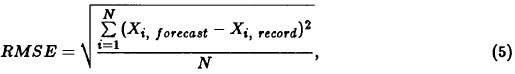
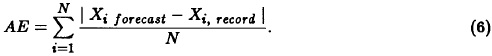
After models are formulated and forecast experiments are performed, validation steps follow. The root mean square error (RMSE), absolute error (AE) and correlation (R) between forecasted recorded values, and skill score (SS) are utilized to evaluate forecast performance (Nicholls 1984; Davis, 1976).

RMSE is defined by

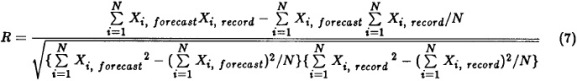
R is a test of the linear relationship between forecasted and recorded value.

SS is an evaluation of the efficiency of a forecasting model, as defined by

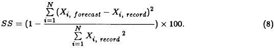
A large value of SS indicates that the model provides reliable forecast values.

4. Teleconnections of OZ climate elements with global SSTs and hemispheric upper air conditions

During the past two decades major El Niño and La Niña events have dominated the global climate pattern, and a substantial effort by the scientific community has been devoted to investigate El Niño/Southern Oscillation (ENSO). Although this study treats SSTs without specifically focusing on the problem of ENSO, the mechanisms involved in ENSO naturally are involved in the manifestation of the teleconnection phenomena that are utilized in regression forecasting. The ways the local SST anomalies in the equatorial Pacific are extended vertically to the tropopause and horizontally to extra tropical latitudes have not been definitely understood. As reviewed by Tribbia (1991), they may involve the east-west Walker circulation, north-south Hadley circulation, wavetrains to disperse stationary Rossly waves, anomalous low level convergence/divergence led by anomalously cold/warm low level convergence, anomalous upper level divergent/convergent flow by anomalous mid level heat release, vorticity transport due to anomalous upper level outflow, etc. As pointed out by Trenberth (1991), however, the tropical Pacific coupled system is fundamentally unstable and multiple possible triggers appear to exist. Thus, the exact trigger of teleconnection may not be pinpointed readily.

Table 1 exemplifies cross-correlation between SSTs and OZ temperature. Very high correlations (|r|≥ 0.8) between OZ January temperature and preceding SSTs are recognized with a significance level greater than 99.9% for the period 1971-85 to 1980-94. Data regions can be identified where preceding SSTs show consistently high correlations (Fig. 3 for data regions). The southwestern Pacific region (SWP) in preceding July is listed eight times. In preceding October and June it is listed seven times and in the preceding September and May it is listed six times. Other preceding SSTs of high occurrence in Table 1 are the Eastern Tropical Atlantic (ETA) in the preceding June and April, the North Central Pacific (NCP) in preceding December and May, the South Central Pacific (SCP) in preceding August and March, SWP in preceding August, and the Southeastern Indian Ocean (SEI) in the preceding September. It is noted that the interannual variations of OZ January temperature are most closely associated with preceding SSTs in the Southern Hemisphere.

High cross-correlations between OZ January temperature and preceding upper air temperatures (T7 and T5), geopotential heights (Z7 and Z5) and geostrophic winds (U7, U5, V7 and V5) are shown in Table 2 for preceding (predictor) months, area of chosen grids and signs of correlation coefficients. The areas whose T7 and/or T5 repeatedly show high cross-correlations with OZ January TMP include Northeastern Atlantic (MEA), Eurasia (ERA), Europe and North Africa (EUA), NCP, Arctic (ARC), Northwestern Atlantic (NWA). Likewise, the areas whose Z7 and/or Z5 show high cross-correlations repeatedly are ARC, NWA and NEA. For V7 and V5, North America (NAM), NWA, ERA and NCP stand out. To exemplify the cross-correlation patterns of the OZ precipitation, significant correlations of January PPT with preceding SST and upper air parameters are presented in Tables 3 and 4. Cross-correlation tables for other months are not specifically presented, but the general patterns are similar as with January TEP and PPT.

The significance and consistency of these spatial and temporal teleconnection patterns justify the construction of regression forecasting models on the basis of such correlations. However, by the very nature of teleconnection study, in no way can such a correlation analysis alone definitively reveal or confirm teleconnection mechanisms involved. In the present analysis it is particularly noteworthy that the Southern Hemisphere SSTs show strong teleconnection with TMT and PPT of OZ, although no Southern Hemisphere upper air parameters are involved in such teleconnections. This seems to indicate that the Southern Hemisphere forcing of SSTs is dispersed to the Northern Hemisphere. Yet, no ready explanation is available for such a mechanism. An anonymous reviewer of this paper comments that stationary waves may be the answer, although a wave triggered in the Southern Hemisphere will meet easterlies in the tropics acting as a barrier, except in the westerly duct region. It is an intriguing question that arises from the present global teleconnection analysis, which demands thorough synoptic-dynamic analyses in the future.

It should be pointed out that all predictors utilized in this study, both SSTs and upper air parameters, are known to undergo interdecadal variations. This is a well-recognized characteristic of the general circulation, but the generally accepted comprehensive theory on this observed fact still does not exist. It is conceivable that both the internal dynamic-thermodynamic processes and the external forcing are involved and interact at various time scales. Among many possible linkages of such non- linear processes, it is most likely the surface and deep ocean currents act through SSTs. The problem is further complicated by the possible forcing of human-induced changes in the atmospheric composition. In the recent review of this problem, Barnett et al. (1999) conclude that recent changes in global climate inferred from surface air temperature are not likely due solely to natural causes, and that at present it is not possible to make a very confident statement about the relative contribution of specific natural and anthropogenic forcing to observed climate change. One essential reason for the use of continuous 15-year data periods for the construction of regression models is indeed to detour this problem at the onset to capture the prevalent modes of variations during the 15 years.

5. MLR and PCR schemes

Using the 15-year data periods 1961-75 through 1980-94, OZ climate elements were predicted for the years beyond the 15-year data periods with multiple linear and principal component regression models. For each month the maximum of 20 MLR and 20 PCR models were formulated for temperature and precipitation for the different 15-year time periods. Table 5 lists the number of models that have selected preceding SSTs and predictands of the previous year as predictors.

SST is selected in all cases of PCR and is the forcing function in the chain of the physical processes to form climate patterns through heat releases to the atmosphere. The PCR scheme is expected to focus in the most fundamental mode of climate variations, and thus it is reasonable to see all PCR cases choose SST as a predictor. Three leading predictors selected for the OZ January PCR models are shown in Table 6. Various upper air patterns are basically a reflection of the SST patterns, and their selection by PCR models is not as overwhelming as SSTs. The recorded value of the predictand in the previous year is also employed for approximately half of the PCR models, representing the persistence of the climatic pattern in their gradual change.

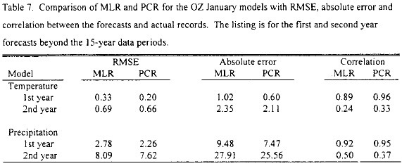
Comparisons of MLR and PCR with OZ January model forecasts for two years beyond the data periods are contained in Table 7. The MLR and PCR are compared in terms of RMSE, absolute error, and correlation between recorded and forecast values. PCR clearly produced better forecast skill than MLR. PCR objectively selects several new orthogonal reference frames among predictors after reducing the problem of multicollinearity, providing more efficient regression coefficients. It is also apparent that the first year forecasts after the data periods are superior to those of the second year. As generally expected, the model deteriorates with time, and deterioration is more serious for the MLR than for the PCR. As will be presented in the next section, the PCR generally retain considerable forecast skill beyond the data periods. For this reason, the forecast experiments presented in the remainder of this paper are only those of the PCR scheme.

6. Forecast experiments

Regression forecast of OZ TMP and PPT were performed with each of the 15-year period datasets from 1961 to 1995. Separate regression models were formulated for TMP and PPT of each month of the year for each data period. The data beyond the 15-year data period were used only as the real time data with the models without updating model coefficients. Forecasts were conducted for all years beyond the 15-year data period whenever the real time data were available.

As listed in Table 6, some predictors appear repeatedly in many 15-year periods throughout the entire data period. For instance, predictor July SST in SWP for OZ temperature is a common predictor from 1967-81 to 1974-88 models. January OZ TMP of the previous year for OZ temperature prediction is another common predictor appearing from 1966-80 to 1968-82 and from 1972-86 to 1974-88. The September SST in NCP is common for OZ precipitation from 1971-85 to 1977-91, as is the December SST in WTP from 1966-80 to 1968-82. The January OZ PPT of the previous year is also common for the OZ precipitation forecast from 1975-89 to 1978-92. The repeated appearance of the same predictors in models may indicate the stability of the scheme and their utility in synoptic analysis.

The performance of OZ temperature and precipitation forecast for up to 10 years beyond the 15-year data period in terms of RMSE and SS is contained in Table 8. The values of RMSE and SS as listed in the table are averages of all models from 1961 to 1994. After the 1970-84 period less than 10 years were available beyond the 15-year period and only the available years were used in averaging. The small values of RMSE and high values of SS indicate high forecast skill. For OZ temperature forecasts, the first forecast years generally show much higher skill scores than those of the second forecast years and beyond. Exceptions are the November and December models, in which the first year forecast skills are slightly lower than those of the second year forecasts for these months, implying a close second year forecast skill with that of the first year. In general, the PCR forecast of the first year after the data period yields a very high forecast skill. This is consistent with the results, as shown in Figures 4 through 11 (5, 6, 7, 8, 9, 10), in which the forecasts for the first years are almost identical as the recorded values. Also as seen in these figures, although somewhat inferior to the forecasts of the first year, the forecasts for the second year and thereafter still generally show a useful level of forecast skill. In precipitation forecast models, the first year forecasts show their RMSE from 1.93 to 14.63 and SS from 61.5 to 98.8, and the second year forecasts show RMSE from 5.49 to 15.67 and SS from 63.3 to 93.7.

Performance of the OZ temperature and precipitation forecasts by PCR, as illustrated for January, April, July, and October in Figures 4 through 11 (5, 6, 7, 8, 9, 10), show the forecast results beyond the respective 15-year data periods and the corresponding recorded values: the former by dots and the latter by lines. The forecasts were performed only for those years beyond the 15-year data periods whose data was the basis of regression formulation; thus the validity of forecast experiment is ensured. The forecasts were not conducted for years where the real-time values for regression models were not available.

The information contained the these figures and Table 8 collectively indicate a considerable level of forecast skill of respective regression models beyond the 15-year data period. This indicates the stability of the PCR regression scheme of this study. It is desirable that the forecast regression models be updated annually by incorporating the data of the current years for the next years. Yet without updating, a reasonable degree of forecast skill still may be expected.

Temperature forecasts, as shown in Figures 4 through 7 (5, 6), are more accurate than precipitation forecasts in Figures 8 through 11 (9, 10). This is expected because of complexity in the precipitation environment and processes. Forecast skill shows some seasonality for some models. For instance, April and July temperature forecasts seem more stable than those of January; and April precipitation forecast seems more accurate than January, July and October. These phenomena are apparently related to the prevailing circulation patterns of the seasons.

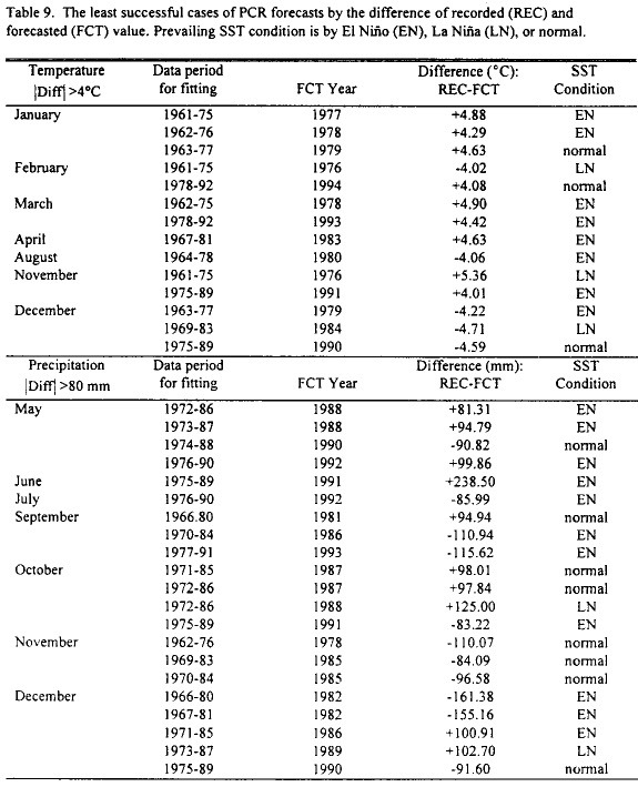
The least successful cases in the forecast as identified by differences between recorded and forecasted value are listed in Table 9. Those cases for OZ temperature are listed for the difference of absolute value of ±4°C or larger. May, June, July, September, and October do not appear in this list for OZ temperature. Eight cases of the total 14 OZ temperature cases are associated with El Niño and two cases with La Niña. The less successful cases in OZ precipitation forecast are those cases of difference with absolute value of ±80 mm or larger. January, February, March, April and August do not appear in the table. Eleven of total 21 OZ precipitation cases for the least successful forecast are also associated with El Niño, and two cases with La Niña. The identification of prevailing conditions of El Niño and La Niña follows the definition by Trenberth (1997). Examination of correlation patterns (for example, Table 1) reveals that most of the strong teleconnections with OZ climate of the Southern Hemisphere occur before the prevalent El Niño period of the late 1980s and 1990s. During the period of El Niño dominance during the last decade, teleconnection with the Southern Hemisphere is very limited. The case study of these less successful cases may be an interesting endeavor in the future.

7. Concluding remarks

The principal component analysis of long-term monthly temperature and precipitation records with a dense observation network over the United States indicates the utility of the principal components to provide the seasonal-range forecast for the region.

The cross-correlation analysis of the OZ temperature and precipitation suggests the useful teleconnection patterns between OZ climate variables and the global antecedent SSTs and upper air circulation. A principal component regression forecasting scheme was constructed in which the predictands were related to their first components that were regressed on antecedent SSTs, upper air parameters and the preceding OZ record. It was shown that the principal component regression scheme is superior to the multiple linear regression scheme.

The forecast experiments were performed for each month of the year with 15-year segments of data for the periods from 1961-75 to 1980-94 for years beyond the 15-year data periods. The examination of the results reveals useful and stable forecasting of the principal component regression models up to 10 years beyond the 15-year data period without significant deterioration of models with time.

The forecast models provide area mean forecast values in the Ozark Highlands area. It should be possible to derive the local forecast by considering the regional differences within the area through additional climate analysis.

Acknowledgments

This research has been supported under the cooperative agreement USDI GS #1445-CA09-95-0069 #2 between Biological Resources Division, U. S. Geological Survey and the University of Missouri-Columbia. The authors are indebted to Dr. G. D. Willson for his comments and consultation, to Dr. W. B. Kurtz for his thorough reading and comments on the manuscript and to the anonymous reviewer whose constructive comments have led to a great improvement of the paper. They also want to thank Mr. H. Kim and Ms. Tanya Akyüz for their technical assistance.

REFERENCES

Barnett, T. P., K. Hasselmann, M. Chelliah, T. Delworth, G. Hegerl, P. Jones, E. Rassmusson, E. Roeckner, C. Ropelewski, B. Santer and S. Tett, 1999. Deletion and attribution of recent climate change: a status report. Bull. Amer. Meteor. Soc., 80, 2631-2659.         [ Links ]

Basilevsky, A., 1994. Statistical Factor Analysis and Related Methods. John Wiley & Sons, Inc., New York, 737pp.         [ Links ]

Blackmon, M. J., J. E. Geisler and E. J. Pitcher, 1983. A general circulation model study of January climate anomaly associated with interannual variation of equatorial Pacific sea surface temperatures. J. Atmos. Sci., 40, 1410-1425.         [ Links ]

Davis, R. E., 1976. Predictability of sea surface temperature and sea level pressure anomalies over the North Pacific Ocean. J. Phys. Oceanogr., 6, 249-266.         [ Links ]

Draper, N. R. and H. Smith, 1981. Applied Regression Analysis. John Wiley & Sons, Inc., New York, 709 pp.         [ Links ]

Geisler, J., M. L. Blackmon, G. T. Bates and S. Muños, 1985. Sensitivity of January climate response to the magnitude and position of equatorial Pacific sea surface temperature anomalies. J. Atmos. Sci., 42, 1037-1049.         [ Links ]

Kung, E. C., and J. -G. Chern, 1994. Large-scale modes of variations in the global sea surface temperatures and Northern Hemisphere tropospheric circulation, Atmósfera, 7, 143-158.         [ Links ]

Kung, E. C., and J. -G. Chern, 1995. Prevailing anomaly patterns of the Global Sea Surface temperatures and tropospheric responses, Atmósfera, 8, 99-114.         [ Links ]

Kung, E. C., and H. Tanaka, 1985. Long-range forecasting of temperature and precipitation with upper air parameters and sea surface temperature in a multiple regression approach. J. Meteor. Soc. Japan, 63, 619-631.         [ Links ]

Kung, E. C., J. -G. Chern, and D. E. Smith, 1995. Global sea surface temperatures and associated long-range predictability of the Northern Hemisphere circulation and local climatological variables. Terrestrial, Atmospheric and Oceanic Sciences, 6, 553-577.         [ Links ]

Kutzbach, J. E., 1967. Empirical eigenvectors of sea-level pressure, surface temperature and precipitation complexes over North America. J. Appl. Meteor., 6, 791-802.         [ Links ]

Lee, J. -W., 1997. Long-Range Variability and Predictability of the Ozark Highlands Climate Elements. Ph. D. Dissertation, University of Missouri-Columbia, 116 pp.         [ Links ]

Montroy, D. L., 1997. Linear relation of central and eastern North American precipitation to tropical sea surface temperature anomalies. J. Climate, 10, 541-557.         [ Links ]

Myers, R. H., 1990. Classical and Modern Regression with Applications. Duxbury Press, Belmont, 488pp.         [ Links ]

NCDC, 1993. Summary of The Month Co-operative T-D 3220, NCDC, Asheville, 29pp.         [ Links ]

Nicholls, N., 1984. The stability of empirical long-range forecast techniques: a case study. J. Climate Appl. Meteor., 23, 143-147.         [ Links ]

Park, C. -K., and E. C. Kung, 1988. Principal components of the North American summer temperature field and the antecedent oceanic and atmospheric condition. J. Meteor. Soc. Japan, 66, 677-690.         [ Links ]

Preisendorfer, R. W., and C. D. Mobley, 1988. Principal Component Analysis in Meteorology and Oceanography. Elsevier, Amsterdam, 425pp.         [ Links ]

Smith T. M., R. W. Reynolds, R. E. Livezey, and D. Stoker, 1996. Reconstruction of historical sea surface temperatures using empirical orthogonal functions. J. Climate, 9, 1403-1420.         [ Links ]

Ting, M., and H. Wang. Summertime U. S. precipitation variability and its relation to Pacific sea surface temperature. J. Climate, 10, 1853-1873.         [ Links ]

Trenberth, K. E., 1997. The definition of El Niño. Bull. Amer. Meteor. Soc., 78, 2771-2777.         [ Links ]

Tribbia, J. J., 1991. The rudimentary theory of atmospheric teleconnections associated with ENSO. Teleconnections Linking Worldwide Climate Anomalies. (M.H. Glantz, R.W. Katz and N. Nicholls, Eds.) Cambridge University Press, 185- 305.         [ Links ]

Unger, D. A., 1996a. Skill assessment strategies for screening regression predictions based on a small sample size. Preprints, Thirteenth Conference on Probability and Statistics in the Atmospheric Sciences. San Francisco, CA, February 21-23, 1996. 260-267        [ Links ]

Unger, D. A., 1996b. Forecasts of surface temperature and precipitation anomalies over the U.S. using screening multiple linear regression. Experimental Long-Lead Forecast Bulletin, 5, 44-45.         [ Links ]

Walsh, J. E. and M. B. Richman, 1981. Seasonality associations between surface temperatures over the United States and the North Pacific Ocean. Mon. Wea. Rev., 109, 767-783.         [ Links ]

Woodruff, S. D., R. J. Slutz, R. L. Jenne and P. M. Steurer, 1987. A comprehensive ocean-atmosphere data set . Bull. Amer. Meteor. Soc., 68, 1239-1250.         [ Links ]