


 nueva página del texto (beta)
 Inglés (pdf)
 Artículo en XML
 Referencias del artículo
 Enviar artículo por email
 Citado por SciELO
  Similares en
SciELO
Similares en
SciELO 
 Permalink
1. Introduction
In Mexico, there are no specific zoning for transportation study issues, such as the Traffic Analysis Zones (TAZ), which are managed in countries such as the United States and Canada to model transportation demand (Department Of Transport U.S, 2021; Sun, 2007). At national level, there is the National Institute of Statistics and Geography (INEGI, by its acronym in spanish), which is in charge of the production and dissemination of geographic information that generates information at some scales, like national, state, municipal, by locality, BGA, electoral section and blocks, in addition of the Mexican Transportation Institute (IMT) that generates and publishes information regarding national transportation, mainly at the state and municipal level, which are the two main scales used in most transportation demand studies (Moreno et al., 2021; Betanzo, 2015; Gradilla & Rico, 2005).
Considering its nature, urban freight transport requires data at the urban, local, or even at establishment level. However, given the aggregation levels of the existing data for transport studies, the Modifiable Areal Unit Problem (MAUP) often arises, which refers to the sensitivity of the statistical and cartographic results, depending on the unit analysis where the data is found. The reason is because the area units are usually subjectively defined and their limits are modifiable (Buzzelli, 2020). This problem is known in the geographical and statistical field, but it is very little analyzed in the study of transport (Briz-Redón et al., 2019). That is why this document aims to show the variability of the descriptive statistical results and some spatial analysis techniques based on different scales of analysis, to model the demand for urban freight transport, in order to deter-mine which of the scales is better to analyze this transport.
To achieve the goal, this document has been divided into four sections. The first one has a literature review on two main topics: the MAUP and, specifically, its consideration in urban freight transport studies. The second one corresponds to the description of the materials and methods used to analyze the effect of the MAUP, at different scales of analysis: BGA, electoral section, and the 500-by-500-meter regular grids, in the variables related to the demand for urban freight transport in the study zone. The third one presents the results of some descrip-tive statistics, such as measures of central tendency, measures of dispersion and distribution, correlation between variables, as well as global and local spatial autocorrelation, obtained in the three scales of analysis. Finally, the fourth one states the final considerations.
1.1 The Modifiable Spatial Unit Problem in spatial analysis
The Modifiable Spatial Unit Problem, also known as the Modifiable Area Unit Problem (MAUP), is related to the fact that the measurements for crosssectional data are sensitive to the levels of aggregation and to the combinations of contiguous units that are made (Anselin, 1988). It is characterized by having two effects, the first is that of scale and refers to variations in the results when considering different aggregations of spatial units, within larger ones, for example: aggregated data in federal entities versus disaggregated data in municipalities. The second effect is that of zoning, which concerns the differences in the results when different unit formations are used, that is, for a fixed number of zones, different aggregation alternatives are used (Vela, 2016).
When the unit of analysis is modified, the data can be regrouped in infinitely new and different arrangements and, therefore, the results and the relationships between the phenomena are different, according to the scale of observation and the spatial extent of the region studied. This difference is evident in the cartographic representation and in the statistical results of the analyzed phenomena because the results of these analyzes depend directly on the definition of the units studied (Buzzelli, 2020).
Some studies that analyze the sensitivity to the MAUP identified that the parame-ters such as the correlation coefficient, univariate statistics, factor analysis, vari-ance, as well as the results and significance in bivariate regression and multiple regression models, vary depending on the number and size of the analysis area (Clark y Avery, 1976; Ravenel, 2003; Xu et al., 2014; Biehl et al., 2018). The MAUP has a direct consequence on the results obtained when executing spatial analysis tools, completely modifying the cartography and the output statistics. This situation occurs mainly in tools whose methods are based on spatial contiguity (maps of discontinuities, local deviations, spatial autocorrelation, measurement of spillover effects, among others) since this is completely dependent on the choice of basic territorial units (Grasland & Madelin, 2006). Therefore, in this paper it was considered important to analyze the sensitivity to MUAP with three methods in particular: descriptive statistics, correlation of variables and spatial autocorrelation, which allow observing the behavior of the data individually, with respect to other variables of analysis and at the spatial level, respectively.
In the past, most studies ignored MAUP effects, as the data and tools to avoid these effects were not available. However, digital cartographic data and Geo-graphic Information Systems make it possible to evaluate the effects of the MAUP and select the optimal units of analysis. Currently, different studies that require spatial analysis have paid special attention to the MAUP. Some the main topics are health studies, vegetation analysis, spatial segregation, relationship between species, among others (Wang & Di, 2020; Nouri et al., 2017; Nielsen & Hennerdal, 2017; Lechner et al., 2012).
1.2 MAUP in urban freight transport studies
The effects of MAUP have received little attention in transportation studies. It has been analyzed mainly in the transport of people, both motorized and non-motorized (Biehl et al., 2018; Mitra & Buliung, 2012), as well as road safety is-sues (Briz-Redón et al., 2019; Xu et al., 2018), in the influence of urban form in the choice of travel mode (Zhang & Kukadia, 2005), as well as in the design of traffic analysis zones (Viegas et al., 2009).
Although urban freight transport has not received as much attention as passenger transport, in recent decades there has been an increasing interest to include spatial variables in its study (Ducret, 2015; Alho & Silva, 2014). These variables are measured at different scales of analysis, which can be macroscopic (at the city or metropolitan level); mesoscopic (at the corridor, neighborhood or local level) and microscopic (establishment level). The microscopic scale has advantages over the other two scales, as it can be more directly related to the explanatory variables and can reflect the behavior of decision makers in freight transport. However, this scale requires estimating the data that are aggregated in the macroscopic and mesoscopic scales (Pani et al., 2019).
The choice of the unit of analysis is mainly determined by the availability of the data, so the results of the models vary depending on the analysis unit used. The variation of results is one of the problems that researchers can face in the modeling of freight transport by the MAUP. The variability in the model parameters is due to the fact that the limits of the analysis units can be modified in infinite ways, which represents a loss of information that changes with each alternative.
Existing studies of urban freight transport modeling have used different analysis units to study this transport. Some have been based on census units (Sánchez-Díaz et al., 2016); municipalities (Cantillo et al., Veras, 2014); regular grids (Du-cret et al., 2016; Alho & Silva, 2014); zones of influence or buffers (Kawamura & Miodonski, 2012); homogeneous industrial sectors (Sahu & Pani, 2020); commercial sectors (Sánchez-Díaz, 2017), and services sectors (Sánchez-Díaz, 2018).
Despite the different scales used to analyze transport, there is not much attention in demonstrating the link between the choice of the unit of analysis and the quality of the model. Here, the model to be described is the one that represents the cargo activity. Freight travel is an induced demand from retail establishments (Rodrigue et al., 2016).
Biehl et al. (2018) mention that, to adequately represent the true relationship between measures of the urban environment and travel demand, the MAUP must be evaluated in the context of several possible spatial representations available, to measure aggregate variables. González and Sánchez (2019) analyzed the impact of the units of analysis and the aggregation of the data in the models of generation of freight transport trips, concluding that the level of disaggregation can influence the quality of the generation rates of freight trips, although not proportionally, so disaggregated estimates generally give more adequate results. Pani et al. (2019) evaluated the impacts of the MAUP effect on load generation models and trip generation models, where they obtained a wide variation in the estimated coefficients in terms of magnitude, statistical significance and direction of association. They concluded that an analyst can design different policy instruments, which can become counterproductive, taking as a reference the effects of the urban environment on freight travel patterns.
2. Methodology
Vector files were used at three different scales of analysis to be able to compare the results, both with some descriptive statistics and when applying different spatial analysis techniques. The three units of analysis were: Basic Geostatistical Area (BGA), which is defined by the National Institute of Statistics and Geography as a geographic area occupied by a set of blocks perfectly delimited by streets, avenues, walkways or any other feature of easy identification on the ground and whose land use is mainly residential, industrial, service providers, commercial, and so on, which are only assigned to the interior of urban areas that are those with a population greater than or equal to 2,500 inhabitants and in the municipal capitals (INEGI, 2020); electoral section, which is defined as the territorial fraction of the single-member Electoral Districts for the registration of citizens in the Electoral Register and in the Nominal Lists of Voters (National Electoral Institute [INE], 2020); and a 500-by-500-meter regular grids, taking as a reference the recommendations of researchers on urban freight transport (Ducret et al., 2016).
The information used to carry out the analysis was the retail businesses in the Metropolitan Area of the City of Toluca, which is in vector format and was obtained from the National Statistical Directory of Economic Units (NSDEU) of the year 2018. The variables selected were the retailers, was chosen as it is considered the main attractive pole for urban freight transport, income, population aged 15 to 64 years, density of primary roads and density of employment per hectare and number of dwellings, as suggested by studies of urban freight transport that include spatial indicators (Ducret et al., 2016; Sánchez-Díaz et al., 2016; Alho & Silva, 2014; Kawamura & Miodonski, 2012). This information was obtained, and in some cases, it was calculated, with the census variables of the 2020 Population and Housing Census, with information from the 2018 NSDEU, and with vector information on the roads in the study area. See Table 1.
Table 1 Variables used
| Variables | Author | Source |
| Retail trade (retail) | Ducret et al., 2016; Sánchez-Díaz et al., 2014 | NSDEU 2018, INEGI |
| Income (income) | Ducret et al., 2016 | Calculated with the 2020 Population and Housing Census, INEGI |
| Population aged 15 to 64 (pop_15_64) | Ducret et al., 2016; Kawamura et al., 2012 | 2020 Population and Housing Census, INEGI |
| Density of primary roads (dens_prim) | Kawamura et al., 2012 | Calculus in QGIS with roadways vector files |
| Density of employment (dens_empl) | Sánchez-Díaz et al., 2014; Kawamura et al., 2012 | Calculated with the 2018 NSDEU |
| Number of dwellings (NumDwe) | Ducret et al., 2016 | 2020 Population and Housing Census, INEGI |
To be able to analyze the effects of the MAUP, in the analysis of the demand for merchandise in the Metropolitan Area of Toluca, several tests were carried out with the variables of interest. These tests consisted of descriptive statistics; cor-relation between variables, as well as global and local spatial autocorrelation (Moran-LISA’s I).
2.1 Descriptive statistics
In this section, statistics of central tendency, dispersion and distribution were specifically analyzed.
In the central tendency statistics, the mean was obtained, which is the sum of all the values of the variable divided by the number of cases, and the median, which reflects the value below where 50% of the cases are found.
Regarding the dispersion statistics, the minimum and maximum values were considered, which is the smallest and largest value respectively of the observed values; the variance, which is a measure of dispersion about the mean, equal to the sum of the squared deviations of the mean divided by the number of cases minus one, as well as the standard deviation (SD), which measures the degree to which the scores of the variable deviates from the mean.
In the distribution statistics, skewness and kurtosis were obtained. Skewness expresses the degree of skewness of the distribution, where positive values indi-cate that the most extreme values are above the mean, while negative skewness indicates that the most extreme values are below the mean. The asymmetry value close to zero indicates symmetry. On the other hand, the kurtosis of the variables is a measure of the degree of existence of outliers that indicates the degree to which a distribution accumulates cases at its extremes, compared to the cases accumulated at the extremes of a normal distribution. A positive kurtosis indicates that the data exhibit more extreme outliers than a normal distribution, while a negative kurtosis indicates that the data exhibit fewer extreme outliers than a normal distribution.
The purpose of obtaining these descriptive statistics is to be able to explore the individual behavior of the data in the three units of analysis, their variation and distribution, which in turn helps to identify the way in which they can be treated later.
2.2 Variables Correlation
Correlation makes it possible to determine the degree of association between variables, that is, the degree to which two variables tend to change at the same time; there are different correlation coefficients such as Pearson's or Spearman's. The first evaluates the linear relationship between two continuous variables and is used when the data have a normal distribution, while the second evaluates the monotonic relationship between two continuous variables that tend to change at the same time, but not necessarily at a constant rate and are used when the distribution of the data is not normal. The correlation can be positive or negative. A positive correlation indicates that one variable increases as another increases, while a negative correlation indicates that while one variable decreases, the other increases and vice versa. Both coefficients take values between -1 and 1, where the zero value, or values close to it, indicates an absence of association of the variables. In this sense, the correlation between the variables of interest in the study area was analyzed in the different analysis units.
Analyzing the correlation coefficient between the variables considered in this study will make it possible to determine how one variable is related to another, and to identify whether this correlation increases or decreases as the scale of analysis is modified, as stated by Openshaw and Taylor (1979).
2.3 Spatial Autocorrelation
Spatial autocorrelation allows identifying how a phenomenon varies across geographic space, to determine spatial patterns and the degree to which local elements are affected by their neighbors. It shows the correlation that exists within the variables through space, where the values observed in a single study variable and the relationship with its closest units are considered (Siabato & Guzmán-Manrique, 2019; Goodchild, 1986). Vilalta (2005) defines it as the concentration or dispersion of the values of a variable on a map. This concept is related to the socalled first law of geography formulated by Waldo Tobler in 1970, which establishes that the closest things in space have a greater relationship than those that are more distant (Tobler, 1970).
Spatial autocorrelation can be positive (when conglomerates or clusters are formed), negative (when they are dispersed); or may not exist when the phenomenon behaves randomly. Spatial autocorrelation is interpreted as a statistical index that allows measuring the degree to which a geographic variable is correlated with itself, in different zones, within the study area.
The Moran Index (I) is one of the most widely used indices to identify the type of pattern that the study variable presents globally. The value of the index I de-pends on the previously established neighborhood criteria, which can be of dif-ferent types: queen, rook, and bishop. These neighborhood criteria take as a reference the movements of the pieces in the game of chess. For the case of this analysis, the queen-type neighborhood criterion was used (Moran, 1950).
The limitation of the Moran Index I to generate global values is sort out by using local indicators of spatial association, better known as LISA, which allow the detection of agglomerations (clusters) and provide a quantification of the degree of significant grouping of similar values around an observation. The sum of the LISA's for all the observations is proportional to the global indicator of spatial association, so it is useful to measure the contribution of each observation to the value of the global contrast (Anselin, 1995).
Spatial autocorrelation, as mentioned by Goodchild (2008), is susceptible to MAUP; analyzing this index allows us to identify which of the units of analysis provides the most relevant information to be represented cartographically, or to be considered in subsequent studies.
2.4 Software
The integration of statistical information to the vector files was carried out with the QGIS software, version 3.10. Statistical and correlation analysis were per-formed in the statistical software SPSS, version 25, and spatial autocorrelation analysis was performed in Geoda version 1.16.0.12.
3. Study zone
The study area is the Metropolitan Area of Toluca (MAT), which is considered the fifth metropolitan area with the largest number of inhabitants in Mexico and the second at the state level. It has a population of approximately two million inhab-itants (National Population Council [CONAPO], 2018). It is located in the central portion of the State of Mexico, to the West of Mexico City, and made up of 15 municipalities. Toluca is the most relevant municipality, given its status as the entity's capital city. See Figure 1.
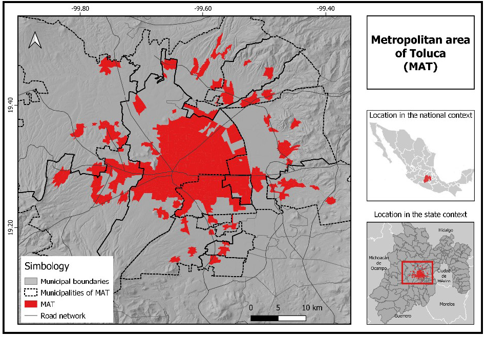
With the industrialization of the area, which emerged in the sixties (Rendón & Godínez, 2016) and the growth of the tertiary sector in the eighties, it is considered one of the most dynamic metropolitan areas in the country. Its economic dynamics is based mainly on the tertiary sector, where practically 90% of the 95,000 economic units in the metropolitan area correspond to this sector. The tertiary sector is made up of 48,000, where 94% of them are retail businesses supplied through urban freight transport, which represents a key aspect that allows inferring the high demand for freight transport trips in the area of study (INEGI, 2018).
4. Results and discussion
This section contains the results obtained that allow identifying the effects of the MAUP in the modeling of the demand for freight transport, using different scales of analysis: BGA, electoral section, and the 500-by-500-meter regular grids.
4.1 Descriptive Statistics
Descriptive statistics, specifically of central tendency, distribution and dispersion, were obtained for the six study variables, in each of the three analysis units.
In the retail trade variable, it can be observed that the central tendency and dis-persion parameters have the lowest values in the grids, while the highest values are in BGA, which allows determining that in the regular grids, the values have less dispersion than in the other two scales of analysis. In the case of the distribution measures, both asymmetry and kurtosis, the three scales have positive values, which indicates that the most extreme values in the three scales are above the mean and that the data in each of they have more extreme outliers than a normal distribution. The scale where this variable has a distribution close to normal is that of the electoral section. See Table 2.
Table 2 Number of retail stores
| Parameters | BGA | Electoral section | Grids 500x500m |
| N | 530 | 660 | 8232 |
| Mean | 32.14 | 26.08 | 7.36 |
| Median | 25.00 | 20.00 | 5.18 |
| SD | 31.69 | 25.648 | 8.15 |
| Varianza | 1004.409 | 657.796 | 66.49 |
| Minimum | 0.00 | 0.00 | 0.00 |
| Maximum | 250.00 | 176 | 142.74 |
| Skewness | 2.137 | 1.834 | 4.316 |
| Kurtosis | 8.302 | 5.647 | 47.360 |
The higher the level of disaggregation, the lower the level of dispersion of the stores, because the grids have smaller dimensions than the other two scales, which makes it possible to notice the concentration of retail stores in the grids. It is worth mentioning that on a BGA scale it is not possible to appreciate, since the extension of this unit of analysis is much greater.
For the case of the others variables, the results obtained are observed in Table 3.
Table 3 Descriptive statistics of the variables of interest
| Income | Population aged 15 to 64 | Density of primary roads | Density of employment | Number of dwellings | |||||||||||
| Parameters | BGA | ES | GR | BGA | ES | GR | BGA | ES | GR | BGA | ES | GR | BGA | ES | GR |
| N | 530 | 660 | 8232 | 530 | 660 | 8232 | 530 | 660 | 8232 | 530 | 660 | 8232 | 530 | 660 | 8232 |
| Mean | 342.4 | 320.7 | 78.3 | 1901.1 | 1921.2 | 434.4 | 9.4 | 10.7 | 1.9 | 12.4 | 21.2 | 10.1 | 694 | 698.1 | 157.4 |
| Median | 293.3 | 253.4 | 38.6 | 1752 | 1653 | 305 | 0 | 0 | 0 | 3.7 | 7.7 | 3 | 663 | 580 | 105 |
| SD | 291.9 | 336 | 104.5 | 1466 | 1417.3 | 446.6 | 21.3 | 24.3 | 8.3 | 26.4 | 45.1 | 22.1 | 523 | 552.3 | 170.5 |
| Varianza | 85192 | 112887 | 10922 | 2149124 | 2008849 | 199454 | 454 | 590 | 68 | 697.3 | 2031 | 488.9 | 273571 | 305005.9 | 29070 |
| Minimum | 0 | 0.1 | 0 | 0 | 9 | 0 | 0 | 0 | 0 | 0 | 0 | 0.00 | 0 | 4 | 0 |
| Maximum | 1969.5 | 5959.1 | 843.9 | 8490 | 20075 | 3553 | 187 | 194 | 148 | 304.3 | 637.6 | 343 | 3328 | 8663 | 1327 |
| Skewness | 1.3 | 8.3 | 2.5 | 0.9 | 4.1 | 1.8 | 3.9 | 3.5 | 6.9 | 6.1 | 6.7 | 6.8 | 0.9 | 5.6 | 1.9 |
| Kurtosis | 2.6 | 123 | 7.8 | 1.1 | 41.8 | 4.4 | 20 | 15.5 | 66.9 | 52.7 | 68.2 | 73.6 | 1.2 | 67.5 | 4.8 |
BGA = Basic Geostatistical Area ES = Electoral Section GR = 500 by 500 meters grids
In the case of income and the population aged 15 to 64, the values for the measures of central tendency are similar in the BGA scale and in the electoral section. In the case of the grids, the values are lower, while in the three scales, the data is scattered, although to a lesser degree in the regular grids. Regarding the distribution statistics, the BGA scale and the grids show a distribution closer to normal, but in the electoral sections, more extreme outliers are appreciated above the mean.
Regarding the density of primary roads, the three scales have the same value in the median, while the mean is lower in the grids. In the dispersion measures, the values are more dispersed in the electoral section scale, while in the grids they have less dispersion. This variable does not show a normal distribution in any of the three scales. The regular grids are the most outliers, above average.
The employment density shows that the values for the measures of central tendency are similar on the BGA and regular grids scales. In the dispersion measures, it is observed that the variable is more dispersed in the electoral section scale. In both BGA and grids, the values are similar. Regarding the distribution, it is observed that in the three analysis scales there is a similar distribution and more outliers, above the mean.
Finally, regarding the total number of dwellings, we have the following: regarding the measures of central tendency, the BGA scale and the electoral section have similar values. Regarding the dispersion measures, the variable is observed less dispersed in the regular grids. Regarding distribution, on the BGA scale, the data have a distribution close to normal. The values furthest from the normal distribution are found on the electoral section scale, where there are also more outliers, above the mean.
As shown by the descriptive statistics, regarding the measures of central tendency and dispersion, the scales that show a more similar behavior of the data are BGA and electoral section, while in the grids a less dispersed behavior of all the variables is observed. The scale, on which a normal distribution of the data can be observed, in most cases, is that of BGA. These results become important indicators of the type of correlation to be used in the next exercise.
4.2 Correlations
With the results of the descriptive statistics, specifically those of distribution, it was possible to identify that the data of each variable analyzed did not show a normal distribution, so the Spearman coefficient was used to obtain the correlation coefficient between variables.
In the BGA scale, the variables that have a significant correlation are retail trade, with the population aged 15 to 64 and total dwellings, the population aged 15 to 64 with income and total dwellings. Income and housing also show a high correlation, but the rest of the variables do not show a significant correlation. See Table 4.
Table 4 Spearman Correlation for BGA´s variables
| Retail | Income | Pop_15_64 | Dens_prim | Dens_empl | NumDwe | |
| Retail | 1.000 | .621** | .834** | .253** | .341** | .797** |
| Income | .621** | 1.000 | .877** | .246** | .355** | .921** |
| Pop_15_64 | .834** | .877** | 1.000 | .165** | .258** | .989** |
| Dens_prim | .253** | .246** | .165** | 1.000 | .301** | .186** |
| Dens_empl | .341** | .355** | .258** | .301** | 1.000 | .271** |
| NumDwe | .797** | .921** | .989** | .186** | .271** | 1.000 |
** The correlation is significant at the 0.01 level (bilateral).
In the electoral section scale, less correlation is observed between the variables. The only ones that show a considerable correlation are income with the population aged 15 to 64 and the total number of dwellings, as well as the population aged 15 to 64 with the total number of dwellings. See Table 5.
Table 5 Spearman Correlation for electoral section variables
| Retail | Income | Pop_15_64 | Dens_prim | Dens_empl | NumDwe | |
| Retail | 1.000 | .517** | .588** | .088* | 0.018 | .567** |
| Income | .517** | 1.000 | .764** | .133** | 0.016 | .814** |
| Pop_15_64 | .588** | .764** | 1.000 | -.144** | -.420** | .988** |
| Dens_prim | .088* | .133** | -.144** | 1.000 | .454** | -.105** |
| Dens_empl | 0.02 | 0.02 | -.420** | .454** | 1.000 | .377** |
| NumDwe | 567** | .814** | .988** | -.105** | -.377** | 1.000 |
** The correlation is significant at the 0.01 level (bilateral).
The 500-by-500-meter regular grids shows similar correlations obtained on the BGA scale; however, a new variable appears to be correlated on this scale, which is that of retail trade with income. It is notable that the correlation coefficients are higher than the ones on the BGA scale. See Table 6.
Table 6 Spearman Correlation for 500-by-500-meter regular grids variables
| Retail | Income | Pop_15_64 | Dens_prim | Dens_empl | NumDwe | |
| Retail | 1.000 | .849** | .924** | .210** | .580** | .900** |
| Income | .849** | 1.000 | .961** | .210** | .579** | .962** |
| Pop_15_64 | .924** | .961** | 1.000 | .195** | .563** | .985** |
| Dens_prim | .210** | .210** | .195** | 1.000 | .259** | .195** |
| Dens_empl | .580** | .579** | .563** | .259** | 1.000 | .564** |
| NumDwe | .900** | .962** | .985** | .195** | .564** | 1.000 |
** The correlation is significant at the 0.01 level (bilateral).
When generating the Spearman correlation matrix with the study variables, it was observed that the most similar correlation values are found in the BGA scales and in the grids, while the variables show less correlation in the electoral sections.
4.3 Spatial Autocorrelation
Moran’s test - global spatial autocorrelation
The results of the Moran Index for the analysis of global spatial autocorrelation of the variables analyzed vary considerably between each analysis unit.
In the case of the retail trade variable, it has a considerable spatial autocorrelation on the grids, so clusters are observed, while on the BGA scale, the spatial distribution pattern is practically random. In the case of the income variable, in the same way as the previous variable, a grouping pattern is observed on the grids scale, while the electoral section has the lowest Moran I, which reflects a more random pattern. The population variable aged 15 to 64 tends to appear grouped in the grids, while in BGA it has a practically random pattern. Regarding the density of primary roads and the density of employment, the highest auto-correlation is observed in the electoral sections, while the other two scales show a weak positive autocorrelation. Finally, the total of dwellings shows a grouping pattern in the grids and a random pattern in BGA. See Table 7.
Table 7 Moran Index
| BGA | Electoral Section | Grid 500X500m | |
| Retails | 0.184 | 0.316 | 0.582 |
| Income | 0.255 | 0.179 | 0.692 |
| Population aged 15 to 64 | 0.073 | 0.235 | 0.628 |
| Density of primary roads | 0.377 | 0.614 | 0.489 |
| Density of employment | 0.524 | 0.620 | 0.520 |
| Number of dwellings | 0.086 | 0.190 | 0.642 |
In conclusion, the global spatial autocorrelation differs in the three analysis scales considerably, being the 500-by-500-meter grids the one that presents the highest global auto-correlation index in almost all the variables. The BGA scale is where a random pattern is observed in most of the variables.
Local Indicators of Spatial Association - LISA
In the case of the local spatial autocorrelation analysis, only was analyzed the retail stores, since it is one of the variables of greatest interest, because it is the attractive pole of urban freight transport, obtaining the spatial groupings and the spatial outliers in the three scales analyzed. See Figure 2.
Spatial groupings (clusters) High-High
They are the clusters that are characterized by having high retail values and that are surrounded by neighboring units with the same characteristics. In this case, significant differences were found in the three analysis scales. 5% of BGAs are in this group, located in the center of the city of Toluca and in practically all the municipal seats of the municipalities that make up the MAT. In the case of elec-toral sections, 9.5% of their polygons have this characteristic. The periphery stands out instead of the center of the city of Toluca, where these clusters are located. Regarding the 500-by-500-meter grids, the high-high clusters represent 11% of the total and are mainly in the downtown area of the city of Toluca.
Low-Low
They are clusters characterized by having a low number of retail businesses, whose neighbors have this characteristic, too. In the case of BGAs, 2% of their polygons are in this category, located mainly in the southern part of the city of Toluca. In the case of the electoral sections, these low-low clusters can be seen to the East and West of the MAT, with 11% of the total polygons. Regarding the grids, 8% corresponds to this type of cluster, standing out in the peripheries of the downtown area of the city, as well as in the neighboring municipalities.
Spatial outliers Low - High
This spatial outlier is characterized by polygons with a low number of retail stores that are surrounded by neighboring polygons with a high number of retailers. The results were as follows: on the BGA scale, these industrial estates represented 2.6% located mainly in neighboring estates of the historic center and some municipal capitals. In the electoral sections, 3.6% have these characteristics and are located on the outskirts of the city center. Finally, in the grids, 0.5% of the polygons are in this category, which are located mainly in the center of the city and in the surroundings of some municipal capitals.
High-Low
In this category are the polygons that have a high number of retail stores and that their contiguous neighbors have a low number of retailers.
In the case of BGA, the polygons with these characteristics represent 1% of the total. They are located to the East and South of the city of Toluca. Similarly, 1% of the polygons of the electoral sections belong to this category, located in the northeast and northwest portion. Regarding the grids, only one of its polygons belongs to this classification and is located to the north of the city.
Corroborating what other researchers have affirmed, regarding the variability of the results, depending on the analysis units, it is evident that in the different scales used, the results vary considerably. This confirms the need to evaluate different scales of work to choose the one that better explains the formulation of proposals that help to improve the urban freight transport, such as regulatory measures or construction of specific infrastructure.
The South-central portion of the city of Toluca and some municipal capitals located to the East and Northwest present coincidences on the BGA and grids scales. The sites that are located on the peripheries of the city center show greater discrepancies, so it is convenient to analyze them with other techniques to determine the optimal scale for the proposal of alternatives in these areas.
It can be concluded that the electoral sections, although at first it seemed to be an ideal scale of analysis due to the continuity of the elements, it is not an adequate scale of analysis, unless it is used as a complementary scale, since the statistical results indicate greater variation. Furthermore, at this scale, none of the variables that were taken for the analysis have a significant correlation with retail stores. The cartographic representation allows to see areas with high-high values that are not observed in the other scales, which can be a valuable contribution. However, there are some units, mainly those in the city center, that are not considered significant and could be underestimated, which would result in limited proposals if only working with this scale.
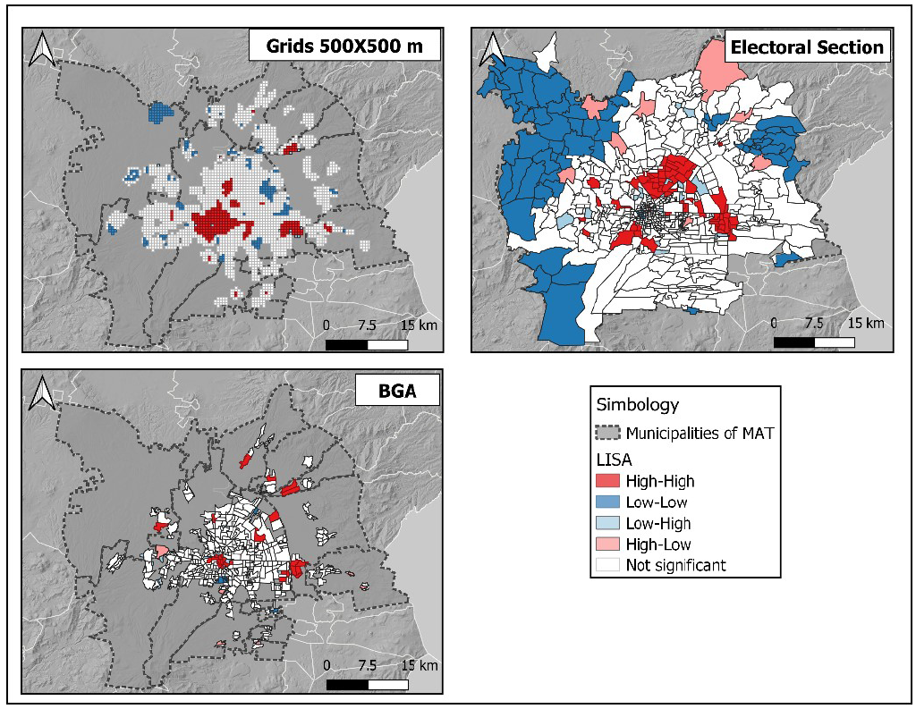
Figure 2 Local spatial autocorrelation of retail stores in the MAT, in three different analysis scales.
The BGA scales and the 500-by-500-meter grids may be the most appropriate to model the transport of merchandise in the study area, since they give the analyst a similar result, reflecting the downtown area of the city of Toluca and the capital cities in most of the suburbs. These sites are the main focus of concentration of retail businesses and therefore attraction poles of freight transport, as well as the correlation of these with some socioeconomic variables, with data that can be empirically corroborated, to generate regulation proposals that can have a greater reach.
The choice of one or another scale suggested in this document will be subject to the availability of data, as well as the level of specificity that is sought. However, there are some advantages and disadvantages on both one scale and another that are worth considering before choosing the final scale. See Table 8.
Table 8 Advantages and disadvantages of the BGA scale and the 500-by-500-meter grids
| BGA | 500-by-500-meter grids | |
| Advantages | ||
| Disadvantages |
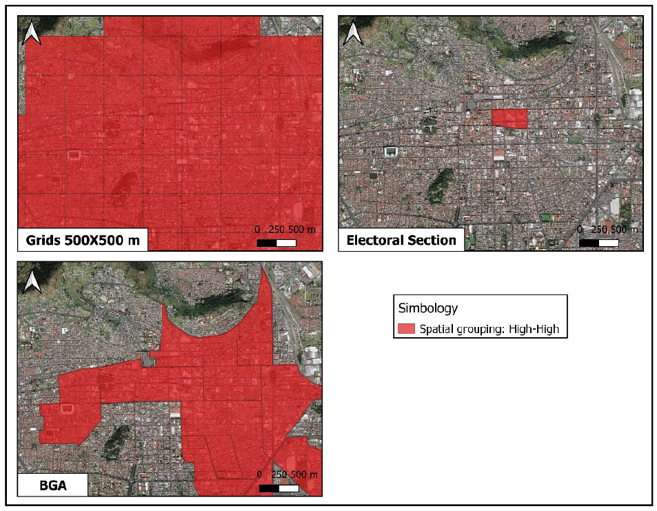
The site that had no discrepancy, regardless of the analysis scale, was the historic center of the city of Toluca, characterized by a high density of employment that is closely related to the mobility of people and goods, as has been observed in other Mexican cities (Chaparro and Hernandez, 2020), making it a priority place in which alternatives regarding regulation and control of this transport can be proposed, as well as the creation of infrastructure to make deliveries more effi-cient and to mitigate negative impacts. See Figure 3.
Working with spatial indicators will always make the researcher wonder about the optimal work scale to carry out any territorial study. Many times, that decision is limited to the availability of spatial data. However, exercises can be done, adding or disaggregating information in different work scales, with the intention of being able to compare the behavior of the data, in each one of them, and determine the impact of the problem of the modifiable spatial unit, with the intention of verifying the sensitivity of the data, when choosing a certain scale of work.
The spatial indicators of the urban environment that were analyzed in this article, such as the number of retail stores, are often added to scales of analysis not suitable for studies of this nature. It is evident that the problem of the modifiable spatial unit results in a wide variation in the estimated parameters of the different variables analyzed, in each of the scales worked.
5. Conclusions
These results make it possible to point out that a researcher can propose differ-ent or even counterproductive alternatives, taking as a reference the results obtained, when considering the demand for freight transport (retail stores) and the socio-territorial characteristics of the study area (population, density of communication channels, employment, housing, income, among many others), at different scales. It can be suggested that the most appropriate analysis scale for the variables analyzed in this document is the grid, since the statistics analyzed show less variation and the correlation between variables is much higher, even the spatial autocorrelation index both globally and locally (specifically in the High-High clusters) is much higher; however, it is advisable not to discard the results obtained in the other two scales, since these can be complementary to identify sites of importance not detected in the grid scale.
This corroborates what Xu et al. (2014); Biehl et al. (2018), Grasland and Madelin (2006) have mentioned about the impact of MUAP on correlation, univariate statistics and spatial contiguity, since it was possible to verify that when changing the unit of analysis the data show different behaviors; in the same way, we agree with González and Sánchez (2019), in concluding that the level of disaggregation influences the results obtained, although not proportionally, and that the units with greater disaggregation give more adequate results.
For this reason, it is advisable to previously analyze different analysis units for the object of study, in order to improve the understanding of the sensitivity of the parameters when changing from one scale to another, with the intention of working on the one that best adapts to the characteristics of the study and, based on them, make proposals for improvement. The recommendation is to learn from the modifiable area units using analysis and representation methods, integrating the multi-scalar dimension and seeing the MAUP not as a "problem", but as a tool to explore the multi-scalar structure of the object of study.
Results in cartographic representations can show changes when modifying the scale of analysis. Each map obtained can be complementary to some other. The results of the statistical analysis, although different, provide knowledge about the behavior of the phenomenon studied.
The results shown in this document are intended to illustrate the need to recon-sider work scales and zoning that may be impacted by the Modifiable Spatial Unit Problem. It is suggested to give continuity to this research, to analyze the results for the same analysis scales with other statistical and spatial analysis tech-niques, such as multiple regression and geographically weighted regression, including the use Artificial Intelligence techniques, which are usually appropriate when there is spatial autocorrelation; or consider other units of analysis different from those analyzed here, which could be grids of different dimensions, or areas obtained from the aggregation of data at the block level to expand the units of analysis offered by official institutions.

