2.1 General Tensile Test Formulation

In a tensile test analysis, by defining the engineering stress value as σ=F/A0 , and the engineering strain value as ɛ=ΔLL0=L-L0L0 where F is the applied force, A0 is the initial area of the tested element, and L0 is the initial length, and L is the final elongation of the tested element (see Fig.1).

The relationships among the ultimate material’s strength Sut , the true stress σt , and the true strain ɛt values (see Fig. 2) on which the proposed method is based, are as follows. Based on both F and A0 , the Sut value is defined as

Therefore, based on the S _ut and ɛ values the true stress value defined as the instantaneous applied stress, at the S _ut coordinate, in terms of the S _ut and ɛ values are determined as

And the true strain value at the S _ut coordinate is given as

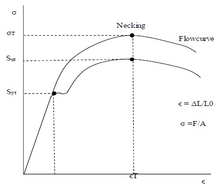
Thus, since now from Eq. (1) the S _ut value can be determined, and from Eq. (2), the corresponding σt value is given, then now let present how the b value is determined.

2.2 Fatigue Slope Formulation

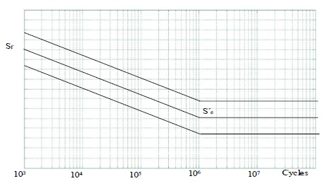
In the analysis, the fatigue slope b value of the S-N curve is the exponent that let us to determine the strength range that corresponds to a desired pair of life cycles values ^[1]. The common approach in the S-N analysis consists in determining b in the logarithm range given by N ₁ = 10³ and N ₂ = 10⁶ cycles (see Fig.3). In this logarithm scale the cycles-strength coordinates to determine b are [log (103),log⁡(fSut)] . and [log⁡106,log⁡Se] Where f represents the strength’s percentage that the material presents after 10³ cycles, and S _e represents the corresponding fatigue strength limit.

Hence, since in this logarithm range the S-N curve behavior is linear given as

Where Y ₁ =log (f S _ut ), Y ₂ =log (S _e ), X ₁ = log (10³) and X ₂ = log (10⁶) then the fatigue b and parameters of the S-N curve are determined as

Therefore, based on Eqs. (5a and 5b) the relation between the applied stress and its corresponding cycles to failure is given by the Basquin formula given as

However, when S _e is unknown, then the fatigue b value defined in Eq.(5a), based on the σt value is given as

Consequently, the cycles to failure defined in Eq.(5c) based on the σt value is given as

Now that from Eq. (5a and 6a) we can determine the b value, let present the methodology to determine the strength Weibull β and η(σ) parameters directly from the S _f and S _e values.

3.1 Generalities of the Weibull distribution

For the two parameter Weibull distribution [⁹] given by

Where t represents the desired life time, β is the shape parameter and η is the scale parameter. However, since in this paper the life of the element is represented by either its cycles to failure N, or by its material’s strength σ value, then by replacing t in Eq. (7) with either N _i or σi , the corresponding Weibull reliability function is given as

From Eq. (8), notice that 1) although to determine the reliability of the element we can use either N _i or σi , the corresponding η(N) and η(σ) values are different ( η(N)≠η(σ) ). And 2) the η(N) and η(σ) values are related by the life/stress model, as can be the Arrhenius, the inverse power law model and the Basquin equation defined here in Eq.(5c). Also notice that because in Weibull analysis, by supposing the failure mode remains constant, then in the ⁿ (N) analysis the β value is considered to be constant ^[10]. Consequently, as shown in Eq. (8), in any Weibull analysis, we always have two Weibull families. One representing the cycles to failure W(β, η(N) ) , and the other representing the material strength W(β, η(σ) ) . Here the analysis is performed based on the W(β, η(σ)) family. Now let present the steps to determine the β and η(σ) parameters directly form the tensile S _f = (f S _ut ) = S _max and (S _e ) = S _min values.

3.2 Steps to Determine the Weibull Strength Parameters

Step1. From the used material determine the corresponding S _ut σt and fatigue slope b values.

Step2. Determine the desired reliability R(n) index to perform the analysis. In practice, it is R(n)=0.9535. And it corresponds to test a set of n=21 parts ^[11]. From ^[11], the relation between R(n) and n is given as

Note 1. Here observe R(n) is not the reliability of the element, instead R(n) is just the reliability on which the analysis will be performed. R(n) is alike the confidence interval CL used in the quality field.

Step3. By using the n value of step 2 in Eq. (10), compute the Y _i elements ^[12] and its corresponding arithmetic mean µy and standard deviation σy values as

Note 2. Observe, once n was selected in step 2, the µy and σy values computed from the Yi elements defined in Eq. (10) are both constant. For n=21 (or R(n)=0.9535) they are µy=-0.54562412 and σy=1.17511694 . In this paper these two values are used.

Step 4. Based on Eq.(6b), by using N ₁ = 10³ and the σt and b values of step1, determine the maximum strength S _f value as

Note 3. Observe that because S _f = f * S _ut , then from Eq. (11) the f value is directly given as f = (S _f )/S _ut .

Step 5. If the S _e value is unknown, then based on Eq.(6b), by using N ₂ = 10⁶ and the σt and b values of step1 determine the minimum strength S _e value as

Step 6. By using the µy value from step 3, and the S _f and S _e values, determine the strength Weibull shape parameters as

Step 7. By using the addressed S _f and S _e values, determine the Weibull scale parameters as

The β and η(σ) parameters determined in steps 6 and 7 are the parameters of the Weibull strength distribution.

Note 4. Notice if f, S _ut , and S _e are known then from Eq.(5a)b can be estimated, implying the true stress σt value is not necessary. It is to say, as shown in Eqs. (13 and 14), the Weibull strength parameters only depends on the S _f and S _e values.

Now based on the β and η(σ) parameters let determine the corresponding log-mean µx and log-standard σx deviation values used to formulate the confidence interval of µx .

3.3 Steps to Determine the Log-mean and the Log-standard Deviation

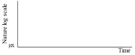
The analysis is based on the linear form of the reliability function ^[2] defined in Eq.(9) given as

Thus, since from Eq. (15) Xi=ln⁡ti , then we need to determine its log-mean µx and its log-standard deviation σx values. From ^[1] the µx value is directly given by the strength scale η(σ) parameters as

And from ^[13], based on both the µy value of step 3, and on the addressed β value, the σx value is given as

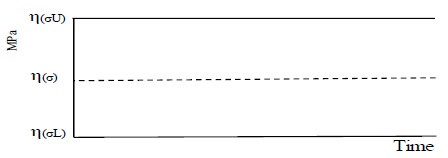
Thus, a confidence interval (CL) of µx is given as

Where Zα/2 is the th desired percentile given by the normal distribution, (which for CL=0.95, is Z0.1/2=1.644853 ).

Unfortunately, although from Eq. (16a) µx=ln⁡(ησ) , the CL limits defined in Eq. (17) cannot be used to determine a confidence interval for η(σ) .

Consequently, Eq. (17) cannot be used to determine the reliability percentiles of the S-N curve neither. This fact occurs because there is not a direct relationship between CL and R(t). CL represents an instantaneous probability that the strength of n identical components behaves around µx , and R(t) represents the probability that a observed (measured) µx value stay around this value through the time. It is to say, while the CL value depends only on the lack of homogeny of the material, the R(t) index depends also on the applied stress, the desired time t, and on the observed µx value. Thus, Eq. (17) should not be used to determine the S-N percentiles that represents the desired R(t) index. Numerically, the deficiency of using CL in reliability analysis is given in section 4.2.

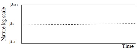
Here notice that in contrast to Eq. (17), in reliability analysis we are interested only in the upper limit. Consequently, since from Eq. (8) the R(t) index depends only on the η(σ) value, then because µx=ln⁡(η(σ)) , in the analysis µx is the lower allowed value that we can used to design the element. Therefore, as shown in ^[14] if µx=ln⁡(η(σ)) is going to be monitored in a process, then in the monitoring control chart the µx value must be set us the lower allowed value.

Now based on the addressed µx and σx values, let present the formulation to determine the reliability percentile of the related S-N curve.

3.4 Reliability Percentiles for the S-N Curve

The efficiency of the proposed method is based on the following two facts.

1) Since from Eq.(14), η(σ) is given as the square root of the product of S _f , and S _e , then in logarithm scale µx=ln⁡(η(σ)) is the average between S _f and S _e , implying that ln⁡(Sf)-ln⁡(ησ)=ln⁡(ησ)-ln⁡(Se) or equivalently that the relation given in Eq.(18) always holds

2) Because in logarithm scale the three values, ln⁡(Sf) , ln⁡(ησ) and ln⁡(Se) , all are in the same S-N line, then this line represents the lower th-reliability percentile for which it is expected the product present the desired R(t) index. Consequently, from Eq. (18) and Eq. (8), we have that the following reliability relationship always holds

Eq. (19) implies that in practice, the derived reliability percentiles of the S-N curve can also be used as the minimum strength η(σi) value that the used material must present to have the desired reliability. Now based on the above two facts, the steps to determine the reliability percentiles of the S-N curve are as follows.

4.1 Weibull Strength Parameters

Step 1. The corresponding strength data are Sut=1515MPa , σt=1655MPa and fatigue slope b=-0.065.

Step 2. Suppose R(n)=0.9535 is desired.

Step 3. The Yi elements are given in Table 1. From these data µy=-0.54562412 and σy=1.17511694 .

Step 4. The maximum strength is Sf=16552*1000-0.065=1009.79MPa .

Step 5. The minimum strength is Se=16552*1000,000-0.065=644.51MPa .

Step 6. The Weibull shape parameter is β=-4*(-0.54562412)0.99*ln⁡(1009.79/644.51)=4.909848 .

Step 7. The Weibull scale parameter is η(σ)=1009.79*644.512=806.7353MPa .

Therefore the Weibull strength distribution to the steel grade (a) A538A (b) material is W(4.909848, 806.7353MPa).

Now based on these parameters let determine the corresponding log-mean µx and log-standard deviation σx values mentioned in section 3.3.

4.2 Log-mean and Log-standard Deviation

From Eq. (16a), the log-mean is µx=ln⁡806.7353=6.692995 and from Eq.(16b) the log-standard deviation is σx=1.175116944.909848=0.239338 , (observe both µx and σx were determined without any observed failure time data). Therefore, from Eq.(17), the 95% confidence interval for µx is CL=6.692995±1.644853*0.239338 ; [6.299319≤µx≤7.086673] or equivalently because from Eq.(16a) µx=ln⁡(η(σ)) , then by taking the exponential, the 95% confidence interval for ησ is [544.2009MPa≤ησ≤1195.9219MPa] , unfortunately as shown next, this confidence interval should not be used in reliability analysis.

For example, notice that although under probabilistic point of view we can say with a confidence level of 95% the lower expected value of the Weibull scale parameter is η(σL)=544.2009MPa , and then it should be monitored in the production process in logarithm scale as in Fig.4 and/or in natural scale as in Fig.5

Unfortunately, as mentioned above in reliability, monitoring (or using) the lower limit of η(σ) is not correct because in reliability the addressed η(σ) value (or nominal µx value) is the lower allowed value. Thus, in the monitoring process, the η(σ) value (or equivalently the µx value) is the one that must be set as the lower allowed limit in the control chart (see Fig.6 and Fig.7).

Additionally, it is shown that although by using the CL limits defined in Eq. (17), the 95% confidence for the S-N curve plotted in Fig.8 is possible, they do not the 95% reliability confidence interval for the S-N curve. Consequently, because the CL confidence interval is not a reliability percentile, then by using the CL values in Eq. (19), the estimated reliability is not the desired R(t)=0.95 index.

Seeing this observe that by using the upper and lower limits of CL to determine R( σ ), the demonstrated reliability is not the desired one. For the upper level η(σU)=1195.9219MPa , then with η(σ)=806.7356MPa in Eq.(19), the estimated reliability instead of be Rσ=0.95 is only R σU=exp-806.73561195.92194.909848=0.8653 .

Similarly, if we use the lower confidence level η(σU)=544.2009MPa with η(σ)=806.7356MPa in Eq.(19), the estimated reliability index instead of be R σ=0.95 , also is only of R σL=exp-544.2009806.73564.909848=0.8653 .

Therefore, the general conclusion is that by using the CL limits in reliability analysis we sub-estimate the real R( σ ) index (0.8653<0.95) of the element, and consequently the CL limits should not be used in the reliability analysis.

Now we know the CL values should not be used, let determine the reliability percentiles for the S-N curve that we can use in any reliability analysis. Following section 3.4.1, the analysis is as follows.

4.3 Reliability Percentiles for the S-N Curve

The reliability percentile analysis for the S-N curve is as follows

Step 1. From Eq.(20a) the upper Yi element for R(t)=0.95 is Yui=ln-(ln 0.95)=-2.970195249 .

Step 2. From Eq.(20b) the lower Yi element for R(t)=0.05 is YLi=ln-(ln 1-0.95)=1.0971887 .

Step 3. From Eq. (21) the upper strength values are

and

Step 4. From Eq. (22) the lower strength values are

and

From the above data, notice because the Yui value was determined by using R σ=0.95 , then by using the Sfu , η(σu) and Seu values in Eq. (19), the reliability percentile is always R σ=0.95 .

For R σ/Sf,Sfu=exp-1009.791849.084.909848=0.95 , R σ/η(σ),η(σu)=exp-806.73561477.264.909848=0.95 , and R σ/Se,Seu=exp-644.511180.204.909848=0.95 .

Similarly, since the YLi value was determined by using R σ=0.05 , then by using the SfL , η(σL) and SeL values in Eq. (19), the reliability percentile in all cases is always R σ=0.05 .

For R σ/Sf,SfL=exp-1009.79807.574.909848=0.05 , R σ/η(σ),η(σL)=exp-806.7356645.184.909848=0.05 and R σ/Se,SeL=exp-644.51515.444.909848=0.05 .

The corresponding percentiles of the S-N curve in MPa and in logarithm scale are all given in Table 2.

Here it is very important to notice from either Table 2 or Figure 9 that data in MPa do not fall in a right line with the η(σ) value.

In contrast observe from Fig. 10 that in logarithm scale they are in line with the η(σ) value. Also notice from Fig.9 and Fig.10 that the upper and lower percentiles are not symmetric around the η(σ) value, and that this fact is due to in Weibull analysis, the η(σ) does not represent the 0.50 percentile, instead it represents the 0.6321 failure percentile, implying the limits around the η(σ) value never will be symmetric around the η(σ) value.

Additionally, remember that as shown in Eq. (18), the symmetrical behavior around η(σ) occurs only for the Sf and Se values from which the η(σ) value was determined. In order to clarify the mentioned facts, in Table 3 the Weibull analysis for the expected values of η(σ) are given.

The practical interpretation of data given in Table 3 is as follows.

1. The values of the column σi in Table 3 represent the maximum applied stress values for which a product that has the η(σ) strength value, will present the reliability R(t) index given in the row of Table 3 that corresponds to the selected σi value. For example, if a component (material) with strength of η(σ)=806.7353MPa , is subjected to constant stress of σ =403.35MPa, then as shown in Table 3, it is expected the element will present a minimum reliability of exp⁡-403.35806.73534.909848=0.9673 . In Table 3, by using the Yi value defined in Eq. (10), the corresponding σi value was determined as

2. The values of the column η(σi) in Table 3, represent the strength value that a product should has to present the given reliability R(t) index when the applied stress is constant at the η(σ) value. For example, the η(σi)=1613.55MPa value given in the first row of Table 3, represents the minimum strength value that a product (material) must have to presents a reliability of Rt=0.9673 when the maximum applied stress is constant at the value of η(σ)=806.7353MPa . It is to say Rt=exp⁡-806.73531613.554.909848=0.9673 . In Table 3, the η(σi) value was determined as

From Table 3 also notice the rows where the Weibull analysis reproduce the Sf=1009.79MPa and Se=644.51MPa values, as well as the upper 95% and lower 5% percentiles of η(σ) were also added. Also from Table 3, notice that as shown in Fig. 9 and in Fig. 10 the behavior around the η(σ) value is not symmetrical. Now let determine the reliability of a component by using the stress/strength analysis.

5.1 Numerical Analysis

In this section, the strength Weibull distribution data addressed in section 4.1 of the steel grade (a) A538A (b) material is used. From this section the addressed Weibull strength family is W (β=4.909848, η_(σ)=806.7353MPa). Therefore, to apply the stress/strength analysis the corresponding stress Weibull distribution must be addressed. Doing this, suppose from an application the maximum principal applied stress is σ1=600MPa and the minimum principal applied stress that generates a failure is σ2=380MPa . ( σ1 and σ2 are the principal stresses given by the Mohr circle analysis).

Thus, with these two principal stress values, from Eq. (14) the scale Weibull stress parameter is ηs=600*3802=447.4935MPa , and from Eq. (13)β=4.909848. Thus, the Weibull stress distribution is Ws(β=4.909848, η_s=477.4935MPa). Consequently, from the Weibull/Weibull stress/strength reliability function ^[1] given as

Therefore, the reliability of the designed component is

Finally, it is important to observe because the reliability index given in Table 3 and that given from Eq. (25) tends to be the same for high reliability indices, (say a reliability above 0.90), then the reliability of an element can be determined directly by using the Weibull strength parameters as in Table 3, or by using the stress and strength distributions in Eq. (25).

Seeing this numerically, suppose that in an application the used material is subjected to reversible stress with Weibull stress parameter η _s =403.35MPa. Therefore, from Eq. (25), as shown in Table 3 , the estimated reliability is

Similarly, if the applied stress is η_s=536.44MPa, then

it is Rt,ηs,ησi=806.73534.909848806.73534.909848+536.444.909848=0.8811 . For detail of the given formulation see ^[1].

Consequently, for high reliability indices, the σi column of any Weibull Strength analysis can be used as the maximum allowed constant stress value that we can apply, in order the component presents the desired reliability. Similarly, the η(σi) column of any Weibull Strength analysis can be used as the minimum allowed strength value that the used material must present, in order the designed element present the desired reliability when it is subjected to a maximum stress value represented by the strength scale η(σ) value. Now by using the proposed Weibull/S-N methodology, the Weibull parameters, the log-mean and log-standard deviation parameters and the 0.95 and 0.05 reliability percentiles of each one of the steel materials given in Table A-23 of the Shigly’s book are all given in Table 4.