


 nueva página del texto (beta)
 Inglés (pdf)
 Artículo en XML
 Referencias del artículo
 Enviar artículo por email
 Citado por SciELO
  Similares en
SciELO
Similares en
SciELO 
 Permalink
Introduction
For an economy with multiple tiers of government, misallocations of tax and spending policies might arise due to coordination failures among different levels of government. In particular, it is well known that a problem of tax coordination could induce vertical (see Keen 1998 and Wilson 1999) and horizontal tax externalities (see Devereuxa et al 2007, among others). Uncoordinated tax policies lead to horizontal fiscal externalities when subnational governments do not recognize that their tax policies affect the tax base of neighborhood districts. This, in turn, could induce state and local governments to overestimate the marginal cost of public funds leading to sub-optimal levels of state and local taxation and spending (see Wilson, 1999). Coordination failures also lead to vertical fiscal externalities because the central government does not take into account how its tax policies affect sub-national tax bases and state and local governments also do not take into account how local taxes affect the tax base of the central government. In this case, all levels of government would underestimate the marginal costs of public funds associated with raising tax revenue leading to high taxation and spending (see Johnson 1988, Boadway and Keen 1996).
Several solutions have been explored to solve the problem of coordination failures for economies with multi-level governments: one possibility is to centralize tax and spending decisions. However, fiscal centralization could actually reduce the national social welfare because the central government might be less efficient than state or local governments in differentiating local taxes and spending according to the inter-regional heterogeneity of preferences (see Oates 1972, Ponce et al 2012). Another possibility is to centralize tax policies but decentralize spending decisions.1 In fact, several countries in the world use some form of tax revenue sharing, a policy that seeks to coordinate tax policies from sub-national governments and the central government, to avoid the negative effects associated with failures of coordination in a federation (see Rao 2007, Kochi and Ponce 2016).
Mexico is one of the countries that have adopted some form of tax revenue sharing as a way to coordinate tax policies from the central and state (same as above) governments. In the particular case of Mexico, the central and state governments signed an agreement to coordinate tax policies in which the central government collects tax revenue that is later distributed among different levels of governments.2
Although there is a large amount of literature that studies the relative merits of fiscal decentralization versus centralization (see Martinez-Vazquez et al 2015 among many others). To the best of our knowledge, there has been little research on the comparative advantages and disadvantages of adopting different fiscal institutions such as fiscal decentralization (in which tax and spending powers are given to sub-national governments) vis-à-vis a tax revenue sharing agreement in which taxation powers are delegated to the central government and (some) spending powers remain at the state level. Since the choice of fiscal institutions affects the provision of local public goods, the effort of the government to redistribute income, fight poverty, and provide important programs such as education and health services that are vital for the citizens´ well-being, it is relevant from a policy making point of view, to have a better understanding of the advantages and shortcomings of these two fiscal institutions.
In this paper we seek to fill in this gap of the literature by developing a comparative analysis of the size and inter-regional distribution of public transfers that would arise under two fiscal institutions: fiscal decentralization versus a tax revenue sharing agreement that seeks to coordinate tax policy among state governments. To be more precise, in this paper we study the optimal allocation of public transfers for an economy that is fiscally decentralized (state governments have full command in deciding the levels of taxation and spending). We also, study the optimal allocation of public transfers for a tax revenue sharing economy: in this economy, state governments and the central government are committed to let the central government design the tax policy. After tax revenue is collected from a given tax base, state governments receive a share of the tax revenue through a formula. We then compare the size and inter-regional distribution of public transfers under these two fiscal institutions.
To do so, we develop several models in which governments are controlled by benevolent social planners that design tax and spending policies to maximize social welfare. In our analysis we distinguish two cases of interest: first, an economy in which local redistribution spending does not show spillovers. Second, an economy in which public spending leads to inter-regional spillovers. The main findings of our analysis are: first, surprisingly, that the effort to redistribute income is the same under fiscal decentralization and tax revenue sharing (that is to say, the nationwide budget for public redistribution is the same for both types of fiscal institutions). This finding is robust and it is observed in economies with and without regional spillovers from public redistribution. Second, the choice of fiscal institutions, decentralization vis-à-vis tax revenue sharing, leads to differences in the public transfers´ regional allocation. We identify conditions in which the size of public transfers in key districts under fiscal decentralization is higher (lower) than those under tax revenue sharing.
Third, in choosing between decentralization and tax revenue sharing as fiscal institutions, there is a tradeoff between the efficiency in the allocation of resources and the inter-regional degree of government effort to redistribute income. This tradeoff could have important implications on regional and national efficacy of the government’s effort to redistribute income. In particular, our findings suggest that if there is a higher (lower) proportion of low income households in some key districts (relative to the proportion of low income households in some other districts) then the government’s redistributive program is more (less) effective in redistributing welfare to the poor under a fiscally decentralized economy relative to the social welfare allotted in a centralized economy with a tax revenue sharing policy.
The rest of the paper is structured as follows: section 2 considers our models of fiscal decentralization and tax revenue sharing for an economy in which there is no spillovers. Section 3 considers the case in which public redistribution shows spillovers. Section 4 includes a comparative social analysis of the choice between decentralization and tax revenue sharing. Section 5 includes a calibration exercise of the model focusing on the inter-regional allocation of resources devoted for redistribution. Section 6 concludes with a discussion of the results and the implications for policy design.
1. Fiscal Decentralization Versus Tax Coordination in Public Redistribution
In the analysis that follows a comparative analysis is developed of the government´s effort to reduce the inequality in income distribution under two different institutional frameworks. First, we consider a government with fiscal decentralization in which policies are uncoordinated (see section 2.1). Second, we analyze government in which there is coordinated agreement on tax policy (see section 2.2). As mentioned before, in this paper we consider tax revenue sharing as an agreement between the central and sub-national governments that seeks to coordinate their tax policies. This kind of agreement has empirical support since countries such as Mexico, India and Pakistan (see Rao 2007) use some form of tax revenue sharing. In the particular case of México, the central and subnational governments signed an agreement to coordinate tax policies in which the central government collects tax revenue that is shared among different levels of governments.3
1.1. Income Taxation and Redistribution under Fiscal Decentralization (Uncoordinated Tax Policies)
In this economy there are two districts
In this economy, the local government in each district sets an income tax
Next, proposition 1 characterizes the equilibrium levels of local taxation and spending for a fiscally decentralized economy.6
Proposition 1. The set of optimal local taxes
Where
Proof.
The problem of tax and redistribution design for a subnational government in
district
In (6)
Re-arrange the first order conditions to show
Use (8) into (9) and then into the local government’s budget constraint to show
Which implies that the national budget on public transfers in the federation,
For an economy with fiscal decentralization, each local government recognizes the
district’s distribution of welfare costs associated with taxation (see condition
7) and the district’s
distribution of social welfare benefits from public transfers (see condition
8). At the equilibrium,
In proposition 1, the equilibrium level of the per-capita transfer for a resident
of district i
2.2. Redistribution under Tax Revenue Sharing (Coordinated Tax Policies)
In this section the equilibrium level of income taxation and public
redistribution with coordinated tax policies for an economy is analyzed. In this
economy, state governments and the central government are committed to letting
the central government design the tax policy. In particular, the central
government sets a uniform
Hence, the problem of policy design for a benevolent social planner at the
central government is to set the income tax
Next, proposition 2 characterizes the equilibrium levels of fiscal policy under tax revenue sharing.
Proposition 2. The optimal tax
Where
The implied public transfers for residents in each district are:
And the national effort to redistribute income in the
federation,
Proof.
The problem of the tax revenue sharing design for an economy with coordinated tax policies in all districts can be characterized by the following Lagrangian
Where
Re-arrange the first order conditions to show
Re-arrange terms from the first order conditions to show that the formulas for tax revenue sharing are characterized as follows:
The implied public transfers for residents in each district are
And the national effort to redistribute income in the economy,
Proposition 2 characterizes the equilibrium levels of taxation and spending for
local governments for an economy with tax coordination and revenue sharing. The
optimal level of the income tax
Moreover, the shares of funds to be allocated in district i,
Propositions 1 and 2 also show that the national budget devoted to redistribute
income by all governments is the same in the equilibrium with fiscally
uncoordinated decentralized tax policies and the equilibrium with tax
coordinated policies, that is,
Since the main distinction in our economy between the choice of fiscal
institutions (decentralization versus tax revenue sharing) relies on the
outcomes of the regional distribution in public transfers, in proposition 3, we
identify conditions in which
Proposition 3
. If
Proof.
From our assumption,
Propositions 1 to 3 show that the choice of fiscal institutions lead to
differences in the regional allocation of public transfers due to the
differences between decentralization and tax revenue sharing in the way that
they aggregate the demands for public redistribution from their citizens.
decentralization and tax revenue sharing aggregate differently the demands for
public redistribution from citizens.12 Moreover, proposition 3 shows that the difference
between the regional distributions of per-capita transfers under fiscal
decentralization vis-à-vis tax revenue sharing depends on the relative
distribution of the household’s social marginal benefits from public
redistribution and the distribution of income.13 In particular, if the share that allocates tax
revenue in district
This outcome might have important implications on the regional and nationwide efficacy of the government’s effort to redistribute income. In particular, this outcome suggests that if there is a higher (lower) proportion of low income households in district i (relative the proportion of low income households in district -i) then the government’s redistributive program could be more (less) effective in redistributing welfare to the poor under a fiscally decentralized economy relative to the social welfare achieved in a centralized economy with a tax revenue sharing policy.
3. Inter-Regional Spillovers from Redistribution
There is a lot of literature in economics that consider the utility of individuals are interdependent (see Bergstrom 1995 among many others).14 If preferences of a household are interdependent then an individual not only cares about his own consumption but also in the consumption of other individuals. In the context of indirect preferences, the well-being of a household not only depends on its own wage, income tax and public transfer but on another household’s wage, income tax and public transfer which might be a resident of district i or district -i. If indirect preferences are interdependent among individuals residing in different districts then public redistribution would lead to inter-regional spillovers (a possibility first analyzed by Pauly 1973).15 The interest of this paper is to analyze, precisely, the role of inter-regional spillovers that leads to coordination failures under fiscal decentralization, while under the tax revenue sharing policy the effect of spillovers will be internalized.16,17
In this case, interdependent indirect preferences are given by
For an economy with tax revenue sharing due to tax coordination, the indirect
preferences for a household with wage w
i
are
Oates (1972) recognized that in a fiscally
decentralized economy, local governments have no incentives to internalize
inter-regional spillovers from redistribution. In this case, it is simple to show
that the equilibrium conditions identified by proposition 1 remain unchanged.
However, for an economy with tax revenue sharing, spillovers will be internalized.
Proposition 4 characterizes the equilibrium tax,
Proposition 4. The optimal tax
Where
The formulas for tax revenue sharing are given by:
The implied public transfers for residents in each district are:
And the national budget for public redistribution
Proof.
The problem of a tax policy design and a tax revenue sharing policy design for an economy with spillovers from redistribution can be characterized by the following Lagrangian
In condition (36),
Where
Re-arrange first order conditions to show
Also re-arrange terms to show that the formulas for tax revenue sharing are:
The implied public transfers for residents in each district are:
Therefore, the national budget for public transfers in the government,
Proposition 4 shows that the equilibrium level of the income tax
An important difference with the model of this section, relative to the model of tax
revenue sharing in section 2.2, is that the share of funds to be allocated in each
district
Proposition 4 also shows that the nationwide budget devoted to redistribute income by
the government for an economy with spillovers from public redistribution is the same
as the equilibrium budget for an economy with tax coordination in which
redistribution does not show spillovers, that is
Proposition 5. If
then
Proof.
See Appendix 1.
Proposition 5 identifies conditions that explain the relative proportion of funds to
be allocated in district i for economies with and without
spillovers from public redistribution. While spillovers from public transfers in
district i create the rationale for an increase in the amount of
resources to be allocated in the district (because spillovers from redistribution
increase the national level of social marginal benefits from public transfers in
district i), the actual formula for the allocation of tax revenue
in district
Next, proposition 6 compares the regional distribution of per-capita transfers between economies with tax revenue sharing and fiscal decentralization for the case in which public transfers show inter-regional spillovers.
Proposition 6 . If
Then
Proof.
From our assumption
then
Since
it follows that
Moreover,
Proposition 6 shows that the difference between the distribution of per-capita
transfers under fiscal decentralization and tax revenue sharing when public
transfers display inter-regional spillovers depends on the relative distribution of
household’s preferences, the distribution of spillovers from public redistribution,
and the distribution of income. If the formula that allocates tax revenue in
district
4. Social Choice Between Decentralization Versus Tax Revenue Sharing
In this section we develop a social welfare analysis of the society’s choice
between decentralization and tax revenue sharing. Our approach is to compare the
society’s welfare under decentralization with the corresponding welfare of the
society under tax revenue sharing. To state the main result of this section, we
define
We also define the ratio
For an economy with tax revenue sharing and no spillovers, the share of resources
devoted for redistribution in the region i,
Lastly, we define
Proposition 7. We define
then decentralization is socially preferred to tax revenue sharing
then tax revenue sharing is socially preferred to decentralization
Proof.
The equilibrium conditions for decentralization are
And the society’s welfare under tax revenue sharing is
Therefore decentralization is preferred to tax revenue sharing if
Where
By definition of a covariance
Define the normalized covariance
Therefore, from (50), (52) and (53),
Proposition 7 says that if the normalized covariance
The intuition behind these results is straightforward: One of the main predictions of our model is that tax revenue sharing will allocate a different amount of resources for public redistribution in each district relative the institution of fiscal decentralization. This means that if we change from tax revenue sharing to decentralization then the size of per capita transfers to the poor corresponding to the local government will increase in some regions and will decrease in other regions. If the per capita transfer increases in region i then the welfare of residents of this district will also increase, which in turn becomes the welfare benefit to motivate a change from a tax revenue sharing policy to a decentralization policy. Simultaneously, if the per capita transfer decreases in other regions, say regions –i, then the welfare of the residents of districts -i will also decrease which in turn becomes the welfare cost to move from tax revenue sharing to decentralization.
Condition (7.2) says that if the
normalized covariance
Similarly, condition (7.1)
identifies examples in which decentralization welfare dominates tax revenue
sharing. An example is that if the normalized covariance
5. Calibration of the Model
In this section we calibrate the model to highlight the differences in the inter-regional allocation of resources to redistribute income under fiscal decentralization and tax revenue sharing. In Table 1, see the Appendix 2, we show the equilibrium conditions of the tax rate, the per-capita public transfer for each state or local government, the size of resources designated for public redistribution in the economy, and the shares of resources for public redistribution allocated in each district for economies with fiscal decentralization and tax revenue sharing. Our model predicts that the tax rates and the size of resources devoted for public redistribution would be the same under decentralization and tax revenue sharing, while the inter-regional allocation would be different under these institutions.20
Our model makes predictions on the per capita transfers in each district and on the shares of resources from redistribution designated to each district. Section 4 also shows that the welfare analysis of the society’s choice between decentralization and tax revenue sharing depends critically on the different allocations between these two fiscal institutions of the shares of resources assigned for public redistribution in each district. Hence the calibration of our model is primarily focused on the shares of resources from redistribution allocated in each district.
As we mentioned before, the ratio
For an economy with tax revenue sharing, the ratio of resources designated for
redistribution in the region i is given by
To do so, we follow the classical treatment on optimal taxation from Atkinson and Stiglitz (1976) and consider
that
Thus, to calibrate the average social marginal income of households in district
i,
In the case of the Paretian distribution, we use the probability distribution function of the Paretian distribution given by
Where
For a comparison of our calibration example between the share of resources for
redistribution allocated at the state level under fiscal decentralization and
tax revenue sharing for an economy without inter regional spillovers see Graph 1 and Table 2 of the Appendix 2.
The share of resources by district under tax revenue sharing,
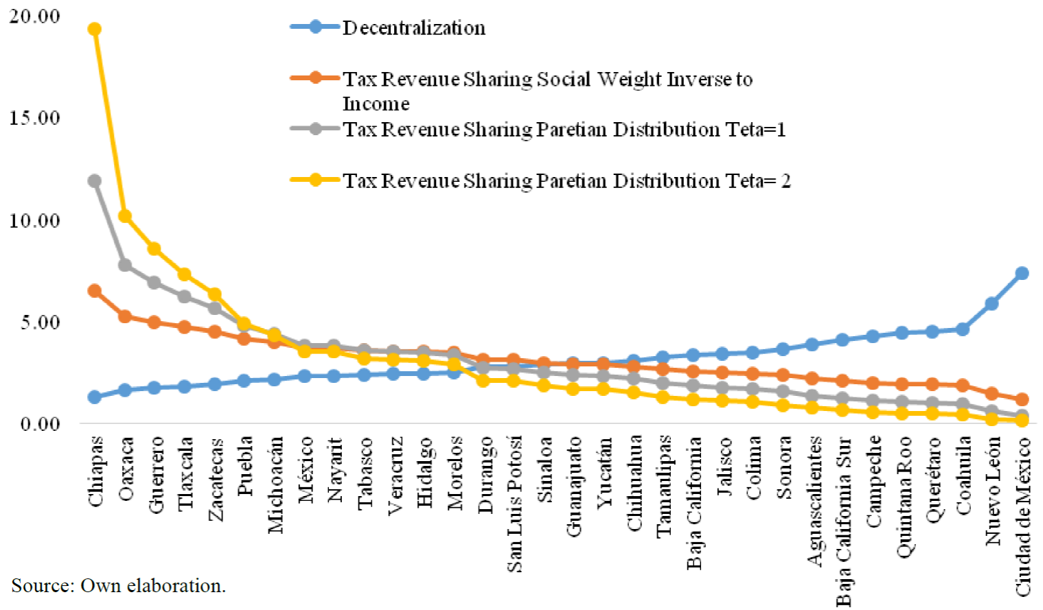
Source: Own elaboration.
Graph 1. Shares of Resources for Redistribution under Decentralization and Tax Revenue Sharing. Case 1: No Inter-Regional Spillovers
Our results show a sharp distinction between the resources allocated for public
redistribution under the institutions of fiscal decentralization and tax revenue
sharing. Under decentralization, the districts with more resources devote a
higher proportion of the economy’s resources for redistribution. This is because
the higher the per capita income in the state, the higher the equilibrium level
of
In contrast to the institution of fiscal decentralization, that will not minimize
the inter-regional inequality of income, under tax revenue sharing the issue of
inter-regional equity becomes an important objective of public policy.
Therefore, an optimal policy of tax revenue sharing will allocate significant
resources to those regions with high social marginal utility of income and,
therefore, more resources might be allocated to districts with low income. The
preference for inter-regional equity is more prominent in the Paretian
distribution with
Under the Paretian distribution with
For an economy with inter regional spillovers we need to estimate the extent of the spillovers. In the context of redistribution, inter-regional spillovers might arise because of an inter-dependence of the well being of households living in different regions (for instance a father who lives in region i who cares for the well being of a relative who lives in region -i and vice versa). In this context, spillovers occur when a household living in region, say -i, receives public transfers and the household living in region i cares about the well being of the household which benefits in region -i from the public redistribution. In this case, we say that there is an spillover effect from the public redistribution implemented in region -i.
In this paper we assume that the higher the population in a state, the higher the chances for the existence of an interdependent utility function with individuals in other regions. This implies, that the higher the population in the state, the higher is the rate of spillovers of that state over other regions. Therefore, we calibrate the extent of inter-regional spillovers from redistribution with the density of population at the state level using data from the “Censo 2010” provided by INEGI. For an economy with inter regional spillovers, our calculations are displayed in Graph two (see below) and in Table 3 in the Appendix 2.
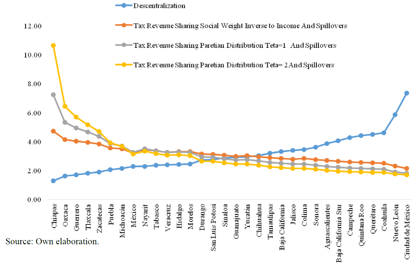
Source: Own elaboration.
Graph 2. Shares of Resources for Redistribution under Decentralization and Tax Revenue. Case 2: With Spillovers
In this economy, fiscal decentralization is a better mechanism to incorporate the inter-regional heterogeneity of preferences for public policy than tax revenue sharing. However, redistribution under tax revenue sharing has two important advantages over decentralization: first, redistribution with spillovers will be Pareto efficient under tax revenue sharing while Pareto inefficient under decentralization. Second, tax revenue sharing leads to a social welfare gain (relative decentralization) due to a more equitable inter-regional allocation of resources.
The distribution of
Under tax revenue sharing with spillovers from redistribution, the three sub
national governments with the lowest per capita income would receive 22.7% of
the economy’s resources for redistribution under the Paretian distribution with
In summary, under fiscal decentralization, the distribution of shares of resources allocated for redistribution is positively related with the state’s own resources. Poor households benefit from a higher amount designated to public redistribution if the household lives in states with high per capita income. In contrast, an equitable allocation of resources across states is an important goal of policy making under tax revenue sharing. Therefore, tax revenue sharing is likely to redistribute more resources to states with lower than average income. As a result, the distribution of shares of resources allocated for redistribution is negatively related with the state’s own resources. Poor households benefit from a higher amount designated to public redistribution if the household lives in states with low per capita income.
The calibration of the model also suggests that there are significant differences in the shares of resources allocated for redistribution for economies with and without spillovers. In particular, our model suggests that, if policy makers take into account not only inter-regional equity but also inter-regional efficiency in the allocation of resources for redistribution, then the amount of resources allotted to redistribution by the states with the lowest per capita income is lower in the case of spillovers relative to the case of no spillovers.
To see this (see Table 4 in the Appendix 2), note that, in the case of no
spillovers, the three sub national governments with the lowest per capita income
would receive 38% of the economy’s resources for redistribution, under the
Paretian distribution with
6. Discussion of the Results and Implications for Policy Design
In this paper we study the size and regional distribution of public transfers with and without spillovers under two different fiscal institutions: fiscal decentralization (in which failures of coordination among sub-national governments might arise) versus tax revenue sharing as a coordination tax policy among different tiers of governments. It is worthwhile to develop such a comparative analysis because it is empirically relevant and, more importantly, because knowing the effect of different forms of fiscal institutions related to the efficiency of the government’s programs would help us to identify potential advantages and shortcomings of feasible policy options.
The main predictions of our theory are the following: first, surprisingly, our models find that the government’s effort to redistribute income (the size of the national budget for public redistribution) is the same for both types of fiscal institutions. This finding is satisfied for economies with and without regional spillovers from public redistribution. Second, the choice of fiscal institutions lead to differences in the regional allocation of public transfers due to the decentralization and tax revenue sharing policies differently aggregating the demands for public redistribution. We show that the distribution of preferences from local spending and the distribution of income explain these differences.
To be more specific, for the case in which public redistribution does not show inter-regional spillovers, the size of public transfers under fiscal decentralization depend only on the average wage of the district while under tax revenue sharing depends on the national average wage and the share of funds to be allocated in the district which is given by the ratio between the distribution of social marginal benefits from public transfers in the district in relation to the national distribution of social marginal benefits. If the share of funds in the district in the tax revenue sharing agreement is lower (higher) than the share of the average wage in the district in relation to the national average wage then the size of the per-capita public transfer received by a resident of the district under fiscal decentralization is higher (lower) than that received under the fiscal institution of tax revenue sharing.
Another relevant implication for policy design in our study is that the optimal formulas for revenue sharing do not depend on the relative contribution of tax revenue of each district (that is, the amount of tax revenue that is collected in each district). This outcome has important implications on the design of formulas for tax revenue sharing because in practice most countries design formulas that take into account how much tax revenue local governments contribute to a general fund. Our paper suggests that the optimal design of formulas should depend only on the district’s relative distribution of marginal benefits in relation to the national marginal benefits of public spending.
In our model in which public transfers show spillovers, fiscal decentralization will not lead to Pareto efficient public transfers while the government’s transfers under tax coordination and revenue sharing are Pareto efficient. Intuition might suggest that because revenue sharing internalizes inter-regional spillovers then the size of public transfers under coordinated tax policies would be higher relative to those transfers under fiscal decentralization. However, this is not necessarily the case. In this paper we identify conditions in which the opposite occurs.
Finally, for the case in which public redistribution shows spillovers, these outcomes suggest a tradeoff between efficiency and the regional size of public transfers.21 This tradeoff could have important implications on the regional and national efficacy of the government’s effort to redistribute income. In particular, if income inequality is concentrated in some key districts then the government’s redistributive program could be more (less) effective in redistributing welfare to the poor under a fiscally decentralized economy relative to the social welfare achieved under a tax revenue sharing agreement.

