


 nueva página del texto (beta)
 Inglés (pdf)
 Artículo en XML
 Referencias del artículo
 Enviar artículo por email
 Citado por SciELO
  Similares en
SciELO
Similares en
SciELO 
 Permalink
Introduction
It is vital for all concerned whit capital market alternatives such as Dimensional Fractal to expand our knowledge on them. One first step would be to describe different existing theoretical models because this would allow to compare while we establish the relevant the securities markets that are related in terms of theory Securities mathematical activity, as in the case of Frankfurt (DAX30), London (TSE), Paris (CAC-40), Tokyo (Nikkie-225) and New York (STANDARD & POOR'S) for Mexico (IPyC). To appreciate the value and diversity of the Dimensional Fractal approach, we believe that the spread of chaos theory and fractal geometry in the social sciences is essential to our future evolution, as the art of storytelling was essential the origins of our culture [Mandelbrot, B: 1999]. There is no rigorous definition with mathematical precision that defines whether a given set or not a fractal. However, most authors agree that Fractal is considered a final product that originates through the iteration of a geometric process. This is usually very simple in nature and originates in the successive iterations sets of certain size, fixed throughout the process that is modified by converting the infinite iteration.
This paper is organized as follows. In Section 1 we contextualize the international Capital Markets according to their type and logistics fractal (mapped and parameterize prices) showing the effects of the non-linearity, reflexivity and the collection of attractors in market functions (cognitive and participation). This Section also considers the price taps geo-fractal iterations for training in Sierpinsky Forks, Cantor and Julia.
In Section 2 we show the geometry of nature in the stock prices, its effect on the topological dimension of study considering the golden mean and the exponent of Hurts. Finally, Section 3 presents the conclusions and recommendations for general use our method.
Definition, Types and Logistics Fractal Capital Market
The term “Fractal comes from the Latin “fractus” meaning “fragmented”, “broken” or simply “torn or broken”. The term is applied to all forms normally generated by a process of repetition wich are characterized by full-scale similarity, not to be differentiable and to exhibit fractional dimensión –. In practical terms, a fractal is a structure that is composed of small parts, which are similar to the original figure, repeated in different scales, from large (macro) to small (micro) [Alligood, K.Yorke, J: 1996]. The fractal approach states that the path from the microcosm to the macrocosm is similar and constitutes a new field of mathematics and is involved in changing the paradigms of science, in our case of the financial economy. The nature expresses itself through its own geometry: Fractals, which is interesting for the analysis of various processes in both nature and society [Shoroeder, F: 2003]. The dynamics of a fractal can lead to a more complicated behavior. For such systems, small differences in initial conditions can grow in large changes in stock values in? markets, where we defines the following recursive propositions referring to stock prices, which are built based on basic financial data:
Role of Participation, relative to market performance:
According to this theory, these two propositions depend on each other and feed each other, and that stock prices vary depending on the information available on the market. This is the sensitivity to initial conditions4 (Ex post price) and it represents one of the attributes of chaos. The pattern is identical to that produced by a random IFS with certain pairs of prices excluded. Others require more excluded combinations (triples, quadruples, etc.). The number of combinations is excluded from this measure of complexity.
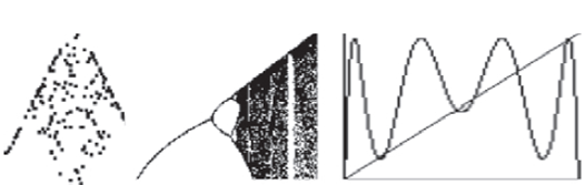
The test functions for our economic and financial dynamics research are the logistic map and the map of the store. The logistic map is defined by a Figure 1.2: Iteration Fractals parabola, the map of the store by a broken line [Diebold, F. Nason J: 1990], both symmetric about x = ½. The height parameter gives the total financial activity, which in our paper is the number of stations that exist in the equity capital markets.
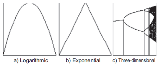
Breaking the map into a discontinuous function the bending of the graph becomes a bifurcation diagram.
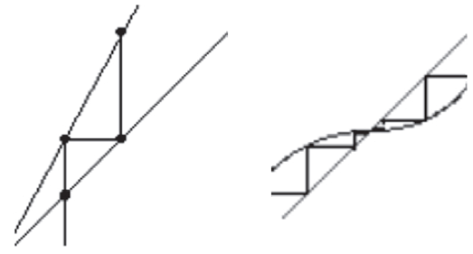
The left side of the diagram resembles the leaf tent (Gaussian), but the left side shows a sequence of periodic windows wich are interwoven in the same order as the disks connected all the cardioid of the Mandelbrot set. Iteration graph of a fractal orbit is produced by generating points (x0, x), (x1, x2), (x2, x3),... in a three-dimensional system:
From x = x0, with a vertical line on the graph y = f (x) from which we repeat function are cut into (x0, f (x)) = (x0, x1), and return to trace the horizontal line (defining market fluctuations) from this point to the diagonal line (defining market trends) y = x, then cut into (x1, x1), to represent the actual price against the logarithmic price [Mandelbrot, B: 1963]. Hence, if we use ln, the price will increase in the short term. The fixed points are the points x * unchanged in the economic and financial dynamics: f (x *) = x * to the sequences generated by iteration of a function of price f (x). For iteration graph, the fixed points are considered intersections y = f (x) y = x.
The loss of predictability is the bad news of the chaos in financial economics, while the good news is a much more robust control of chaotic systems in the stock market. Under occasional slight changes in the price of stock system, it is possible to stabilize any of unstable periodic orbits pervading chaos. Each point of the orbit is in a drawer (or time), and as it follows in the orbit (market trend) it increases each point of the horizontal line. Then, it is possible to determine an approximate measure of the amount of time keeping that passes into the orbit of each price region5. The starting point is an original information which is then processed to obtain the result. This is processed again (iterates) and one obtains another similar result to the above and continues doing the same procedure indefinitely with each outcome. The Hausdorff-Besicovitch dimension6 is:
Where S is the number of segments or their length, L is the measuring scale; D is exactly the size, then we obtain:
By using properties of logarithms we can say that:
Finally we divide both sides by log L and obtain:
Triangle on triangle to the limit of any imagination, the curve thus constructed is undrawble, as the contour shape is repeated at all levels. Each point on it, if we explore it with a magnifying glass, we always reveal the same secrets; triangle on triangle, indefinitely [Batten, J. Ellis, C:1996]. In organizations like the ones analyzed here, this process is called self-similar, since each of its parts is equal to the total (they look the same at any scale) and from the mathematical point of view it has certain peculiar properties that distinguish representation as follows [Briggs, J:1990]:
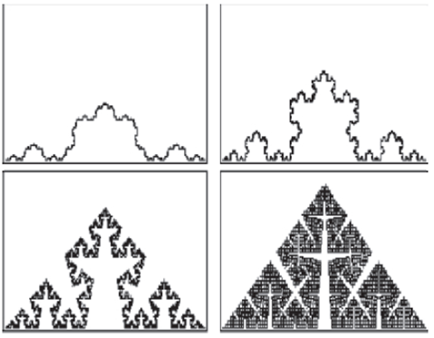
The outline of the Koch snowflake is so irregular that between any two points on it there is an infinite distance and countless cracks and zigzags. The latter makes it impossible to draw a tangent (straight play, uncut, to the curve at a single point) somewhere along its perimeter. Take a line of length L=1m, for example, and divide it into three equal pieces of l = 1/3 m long. In this case, the number of partitions which are generated (N) is obtained by determining how many times does the one hand Ll in total: N = L / l = (L / l) 1 = 3. If we repeat the process on the blade paper to which we consider as a square of side L=1m, which we cut into smaller squares of side l=l/2m and area l²=1/4 m², the number of partitions is now N=L²/l²;= (L/l)²=4. Then the iteration is well symbolize: xn+1=x2n and when applied to any initial value, for example, x0=2, the first calculation would be x1 = (2) 2 = 4, then x2 = (4) 2 = 16 and x3 = (16) 2 = 256, and so on. If the initial value chosen is different, x = 0.5, for example, the orbit will be: 0.5-0.25-0.0625-0.00390625-... ∞, and the attractor is 0. Self-similarity and self-affinity are concepts that unify areas as fractals, power law and chaos.
The self-similarity or invariance under changes of scale or size is isotropic. The self-similarity is one of the fundamental symmetries that govern the universe and an attribute of an infinity of the phenomena.
The distances between the doubling time of successive bifurcations lead to the discovery of a new type of scale. The price in an N-cycle becomes unstable, a stable cycle appears 2N: each point in the cycle results in two points of the 2N-cycle. As the price continues to rise, the 2N-cycle becomes unstable, and each point gives rise to two points of a stable-4N cycle, and so on (in a two dimensional plane).
Geometry of nature in the share prices
One approach to characterize and classify objects even for fractals is attributed to each a numerical quantity, the fractal dimension. Through this mathematical index it is possible to quantify the geometry of objects or fractal phenomena. One interpretation of the dimension, possibly the most natural, is related to the ability of objects to fill the Euclidean space in which they are located.
The dimension will assist in determining the contents of fractal sets. Thus, fractal measure will define, for any procedure, the proportion of physical space that is filled by them. We found a major difference from Euclidean objects: if we magnify an object on Euclidean “dimensional” look straight segments [Sidney, A: 1961]. However, if we successively magnify a fractal object, objects found complication levels comparable to those of the starting set. Mathematical processes to create fractal geometry are iterations of order “n”. The essence of fractals is the “feedback”. The starting point is Capital Market information is processed and one can get indexed. This is processed again (iterates) and one gets another price range similar to the above and continues doing the same indefinitely with each stock price. The similarity or scaling transformation consists in generating a similar copy of any share price on a different scale. To accomplish this, Ex ante price should be affected by a factor of proportionality (the price delta = 3), that is called scaling factor7. Thus, two prices (Ex ante and ex post) are similar if they have the same geometry, but have different values and number of shares used. This can be expressed in a general way, and if we choose a price and model it with logs and amplified by a scaling factor delta, there is a geometry identical to the rank8 price (maximum price, minimum price). Taking the latter range and amplified again by the same scaling factor it is possible to obtain a geometry similar to the price ex ante. This operation can be repeated indefinitely.
The property of self-similarity in a fractal-Dimensional occurs throughout the range of scales [Dacarogna, M. Ramazan, G: 2001]. The self-similar fractals are structures that remain invariant to changes in scale -they have the same properties in all directions-, and they remain invariant when scaled uniformly in all directions. Let's now form a sequence of numbers in order to demonstrate the self-similarity in the following manner. Let's start with zero and one, if we add gives:
Now we add the 1 on the right with the previous one on the left side:
Now add this 2 in 1 which is on the left, before the equal sign:
And we form the sequence, adding the result with the last number on the left side:
And so on. This will form the Fibonacci sequence, which is:
This sequence has very interesting arithmetic features with important applications, as we will see below. First, by multiplying each number in the sequence by 1.6., this gives the following sequence:
If now we round each of these numbers to the nearest integer are:
That is precisely the Fibonacci sequence! (except for a few initial terms and possibly later). In other words, it turns out that the Fibonacci sequence is self-similar and therefore fractional [Guzmán, M., Martín, Morán, M., Reyes, M: 1993].
A fractal object is expected to self-affine when remains invariant under a transformation scale called anisotropic (different scales in all directions). If one zoom the object, one of the coordinate axes becomes a factor b, x →bx, the rest of the coordinate axes need to be rescaled by a factor b ai , x i → b ai x i in order to preserve the invariant set. The exponents ái are called exponents of Hurst and inform us what is the degree of anisotropy of the whole.
The demonstration of self-affinity i s demonstrated as follows: We take a number of the Fibonacci sequence and then divide it as follows below [Talanquer, V: 1996]. If we start with the second, which is 1, and divide by the third, which is also 1, gives:
Now divide the third, which is 1, between the fourth, which is 2, and gives us:
Dividing the room, which is 2, between the fifth, which is 3, gives:
If we thus obtain the following numbers:
If we continue this process we realize that all other ratios are closer to 0.618. The latter is called the golden mean. Another way to get it is as follows: We add 1 to 1, which gives us 2. Take the inverse:
We add 1 to this number:
Take the inverse:
So far, we have the following operation:
Now repeat the procedure with 0,666. We add 1, which gives us 1,666 and take its inverse:
Note that what has been done so far:
Continuing with this we obtain the following ways. We add 1 to 0.6 and get 1.6. Its inverse is:
This value can also be written as:
If this procedure is continued the result becomes a time when the number 0.618 is obtained. Continuing, we add 1 to get 1.618.
Its inverse is:
0,618 Again! Therefore, to continue the procedure 0,618 will be obtain all the time. We started with a series of time t, and observations:
Where:
X t ,N = |
Cumulative deviation over N periods. |
e u = |
Incoming flow in the year u. |
M N = |
Average e u over N periods. |
The range is then converted into the difference between the maximum and minimum achieved as follows:
To compare the different types of time series, Hurst divided this range by the standard deviation of the original observations. This new scale range should increase with time. Hurst made the? following relation:
Where:
R/S = |
range with the new scale. |
N = |
number of observations. |
a = |
a constant. |
H = |
Hurst exponent. |
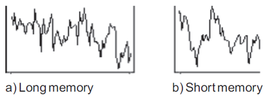
events have greater impact than more distant but still, the latter still have some residual effect. On a larger scale, an event that exhibits Hurst statistics is the result of an influx of interconnected events. What happens today influence the future. Where we are now is a result of where we were in the past. Timing is important. As you throw a pebble into the water, the events of today are drowning in time. The waves that were produced by passing the water fade until, for any reason or purpose, the waves fade [Romero, G .Ojeda, R: 2004].
Conclusions
In this paper we showed that the instruments of Method-Dimensional Fractal exhibit the property of non-linearity as there is no proportion between cause and effect and the lack of temporal linearity is evident. For example, by being a story and just days or months later is when it comes to be taken into account as one needs to define the times Ex Ante and Ex Post, markets overreact or also go to the other end and play “the dead”. Hence three possible causes explain the repeated distortions: emotions including fear and greed, information asymmetries and irrational behavior of the agents as reported by the Behavioral Finance. They all conspire against the linearity and each is worthy of an essay in its own right. Chaotic phenomena are fed themselves as in the case of a hurricane. Markets also feed back to themselves; the more insistent is a movement upward or downward. More people are willingness to participate reinforcing the path and the greater the intensity of the movement, the greater the feedback to reach absurd levels as in a collapse (crash) or a speculative bubble.
The simplest attractor is the market average, the values may be dispersed but tend to return to around the average. Hence, assuming that markets respond to a Type chaotic then we talk about creating Fractals Markets. It is relevant to remember that a stable system tends over time to a point, or orbit, according to their size (attractor or sink) .The score of a fractal is the plot of the values of the orbit in order. That is the graph of points (0, x0), (1, x1), (2, x2),... When representing many points, the order can be emphasized by drawing lines connecting successive points.
This is one of the most common ways to display the temporal patterns of stock prices which are obtained first by dividing the range (highest price/lowest price) represented vertically to be consistent with the iteration graph.
If the log parameter in the stock market increases, there will be a reduction in the price effect resulting in a couple of points, one stable, one unstable, and this depends on the number of shares outstanding and price ranges. This tangent bifurcations lead to a couple of cycles, one stable, the instability of another, so the demand for methods Fractals, claiming in mind that the essence of new fractals is the “feedback”. The implications of the theorem are amazing, simply apply the iteration at one point, the z0 = (0, 0), to determine the nature of the Julia set will be obtained when the iteration is applied to the whole complex plane and in the process of division with golden mean and the number of sections generated is given by N=(L/l)df, where d is what I call the Hausdorff dimension of the object. It should be noted that the same relationship must be true whether we decided to section the whole object and any part there of (whether of the market at the station or vice versa). The mathematical processes that create the fractal structures are iterations of simple rules in considering initial objects at all times to mitigate the logarithmic modeling.
Contributions
With Fractal geometry it is possible to represent infinite number of irregular shapes, non-linear, which at the end to represent rough objects. For this reason, Fractal geometry is the ideal medium in the study of phenomena characterized by complexity and allows us to analyze three observations:
There are additional dimensions to the stock prices in Mexico and the World logarithmic effectively with ln 10 or closer to reality compared with Euclidean geometry which considers only a perfect market and impossible to prove (no balance).
Most prices are complex systems in the volume of buying and selling, but also chaotic due to the issuance of shares outstanding as they exhibit strange behaviors associated with boundaries or fields that cannot be represented in whole dimensions. This means that the average price ranges are fractional (is broken and is fractal).
Fractals are scalable, that is, they can reduce or extend the analysis to see details for the logarithm of a number in a given base. It is the exponent which must raise the base to get the number and mathematical function; and it is the inverse of the exponential function, while the basic forms are preserved at each price level (price high, low, etc.).
According to statistical mechanics, Hurts rate should equal 0.50 if the series is a random path. In other words, the range of cumulative deviations should increase with the square root of time, N. When H is different from 0.50, the observations are not independent; each observation has a memory of all events that precede it. This was not a short-term memory, which is usually called Markovian and is another evidence to use our method.

