


 nueva página del texto (beta)
 Inglés (pdf)
 Artículo en XML
 Referencias del artículo
 Enviar artículo por email
 Citado por SciELO
  Similares en
SciELO
Similares en
SciELO 
 Permalink
Introduction
The objective of optimal diversification is sought by portfolio managers and studied in the literature. Its complexity sometimes clashes with the objectives of return, risk and degree of investor aversion. Finding the perfect mix across different markets, there is no consensus in the literature, as will be seen below. Optimizing portfolios where there are multiple objectives, including diversification, leads to problems with objective functions that may have multiple local optima. Barkhagen et al., (2019) present two global optimization algorithms for such problems. But not to mention the limits of this optimization, in terms of the minimum number of assets to be used. The objective of this paper is to study the level of diversification in an investment portfolio using the Treynor-Black model. It is limited to observe and study when the portfolio contains few assets and a higher percentage of the invested capital, since a low correlation does not impact the level of diversification as much as the number of assets and the dispersion of capital in these assets. Under the assumption that the Treynor-Black model only seeks to weight more capital in assets with better performance (as measured by appraisal, explained below), it does not consider the whole investment as a diversified portfolio.
Not only correlation and volatility can offset the risks in an investment portfolio. But also, the amount of assets and the proportions of investment in each of them. Woerheide & Persson (1992) study five different measures of diversification in an investment portfolio. They found that the complement of Herfindahl index is the best of those analyzed (used in this paper). Being the benefits of diversification of a portfolio is the reduction of risk, it is not the improvement of performance. Although there are studies that mention that diversification can help outperform the benchmark. For example, Banner et al., (2019) found that more diversifications can outperform the benchmark because these portfolios have a higher abnormal return, derived from a higher variance, related to small stocks not contained in the benchmark.
Improve diversification through better risk management. Although its difficulty may be associated with different factors to consider. Fragkiskos (2014) and Shari et al., (2019) can be consulted with the different factors to consider in diversification. Fleming (2021) presents an optimization method that maximizes diversification and minimizes risk instability, through kurtosis. As in previous works, they do not mention the minimum number of assets to achieve it.
Another way to improve diversification is to invest in different sectors. Between 40% to 60% of diversifiable risk can be eliminated (Frahm & Wiechers, 2011). But the limits of this diversification, in terms of the minimum or optimal number of assets to use, are not clear. Benjelloun (2011) surveys the literature seeking to answer the question how many stocks can achieve diversification? He concludes that with 40 to 50 stocks diversification can be achieved. Contrary to Bhuyan, et al., (2016) conclude that equally weighted naïve portfolios should have between 9 to 15 assets to achieve better diversification. And no definite number of assets was found in the differently weighted portfolios to achieve similar diversification. Raju et al., (2021) demonstrates in the Indian stock market, with a portfolio of between 40 to 50 stocks, one has a diversified portfolio that can reduce diversifiable risk by 90%, with 90% confidence.
The objective of this paper is to analyze the diversification offered by the Treynor-Black model in its active part. The study involves the analysis of portfolios formed with this methodology using the components of the DJIA, between 2000-2020. Since this model can offer on average an abnormal return of 6% above the DJIA return, with a probability of outperformance of 66.9% (Samaniego, 2022). They conclude that its performance, measured by appraisal ratio, is superior to the DJIA and other optimization methods used in the literature (equal weighting, mean-variance, semi-variance, maximum Treynor-Black omega in its two components, among others). These results are high, according to Cuthbertson et al., (2010). They suggest that between 2%-5% of equity mutual funds in the UK and USA outperform benchmark indices and between 20%-40% have low returns.
I. Methodology
The Treynor-Black model (1973) is used in its active part. The proposed model is through the investment of two types of portfolios: active and passive. The passive portfolio is the investment in the benchmark and the active portfolio is the investment in assets with positive alphas, obtained through the CAPM model (see equation 1). In equation 1, returns are calculated by rolling windows in annual periods. Only models with R^2
In this paper only the active portfolio will be used, as Samaniego (2022). Due to the results obtained by the authors, in 5 134 simulations. The active portfolio weights its assets based on its appraisal. See equation 2 for the calculation of the weighting and equation 3 for the appraisal calculation.
To measure the value of diversification, Woerheide & Persson (1992) use the adequacy of the Herfindahl index (see equation 4). The variable
These 4 equations are used in each observation (5 134) for each of the 30 assets belonging to the DJIA at each moment. The DJIA between 2000-2020 has had 57 assets, during each observation the 30 assets belonging to the DJIA are selected and their alphas are calculated using equation 1. Only in the cases of having a positive alpha is their appraisal calculated, using equation 3. See Figure 1 for all calculation. The data are obtained from FactSet and processed in Matlab.
Results
Figure 2 shows the number of assets (horizontal axis) contained in the portfolios formed with the Treynor-Black model, in relation to the annual return (vertical axis). The distribution of returns is in black for the TB and the DJIA return (red) is placed next to it. The best distribution of returns for the TB is found when portfolios are assembled with 12 and 13 assets.
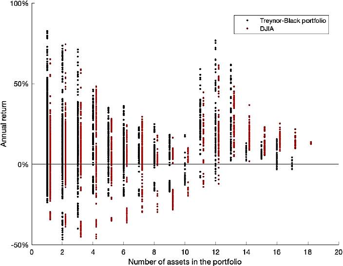
Source: own elaboration and data from FactSet.
Figure 2 Comparison of annual returns in relation to the amount of assets in the TB portfolio
It would be expected that the higher the level of diversification, as measured by equation 4, the lower the number of negative returns, caused by a higher level of diversification. Looking at Figure 3 and figure 4, there is no clear trend of improvement. Since the best portfolios are found at both extremes (H=0, H>0.85).
Source: own elaboration and data from FactSet.
Figure 3 Diversification levels with the complement of the Herfindahl index
Source: own elaboration and data from FactSet.
Figure 4 Diversification levels with the complement of the Herfindahl index>0.85.
Looking more closely at returns when H>0.85 (see Figure 5), although there are few observations with returns below 0%. Visually it is not possible to determine who has the better performance, DJIA or TB. The histograms of the yields in Figures 5 and 6, with H<0.05 and H>0.85 respectively. Clearly the superiority of TB with H<0.05 and DJIA with H>0.85 is observed. The problem with TB with H<0.05 is that it is only invested in one asset. The statistical results are discussed below.
Source: own elaboration and data from FactSet.
Figure 5 Distribution of annual yields using the complement of Herfindahl index>0.85
Source: own elaboration and data from FactSet.
Figure 6 Distribution of annual yields using the complement of Herfindahl index<0.05
Table 1 shows portfolios with different amounts of assets, favoring the highest quality of assets in the portfolio. The more assets in the portfolio, the more diversification we would expect, which would translate into a lower probability of negative returns. This is achieved up to 14-17 assets in the portfolio, but the probability of outperforming the DJIA and the average return is lost.
Table 1 Probability of outperforming the DJIA: it is favorable to have a greater amount of assets
| Assets in TB | TB average annual return (a) |
DJIA average annual return (b) |
(a)-(b) | TB min. annual return |
DJIA min. annual return |
Observations | Probability TB>DJIA |
Probability TB>0% |
| 1 to 17 | 13.8% | 7.8% | 6.0% | -39.1% | -46.2% | 3 435 | 66.9% | 84.2% |
| 2 to 17 | 12.3% | 8.7% | 3.6% | -39.1% | -46.2% | 2 372 | 59.6% | 83.7% |
| 3 to 17 | 11.0% | 8.7% | 2.4% | -39.1% | -46.2% | 1 884 | 57.5% | 82.7% |
| 4 to 17 | 11.0% | 9.1% | 1.9% | -39.1% | -46.2% | 1 482 | 57.5% | 82.7% |
| 5 to 17 | 11.1% | 8.9% | 2.2% | -36.2% | -36.4% | 1 208 | 61.3% | 83.7% |
| 6 to 17 | 10.8% | 9.2% | 1.6% | -24.5% | -36.4% | 996 | 59.5% | 82.8% |
| 7 to 17 | 12.1% | 11.0% | 1.1% | -17.6% | -29.7% | 826 | 59.9% | 84.7% |
| 8 to 17 | 12.8% | 12.6% | 0.2% | -17.6% | -29.7% | 646 | 56.8% | 83.3% |
| 9 to 17 | 13.5% | 13.5% | -0.1% | -17.2% | -28.2% | 600 | 54.2% | 83.3% |
| 10 to 17 | 16.3% | 17.2% | -1.0% | -14.4% | -19.6% | 503 | 47.3% | 89.3% |
| 11 to 17 | 17.5% | 18.6% | -1.0% | -11.5% | -14.1% | 466 | 47.2% | 90.3% |
| 12 to 17 | 17.4% | 19.2% | -1.7% | -10.1% | -12.2% | 410 | 43.2% | 92.0% |
| 13 to 17 | 14.8% | 18.5% | -3.6% | -3.2% | 1.8% | 292 | 28.8% | 93.8% |
| 14 to 17 | 8.0% | 14.8% | -6.8% | -3.2% | 1.8% | 201 | 9.0% | 91.0% |
| 15 to 17 | 5.9% | 13.5% | -7.5% | -3.2% | 5.5% | 147 | 0.0% | 87.8% |
| 16 to 17 | 3.7% | 15.0% | -11.2% | -3.2% | 8.2% | 69 | 0.0% | 73.9% |
Source: own elaboration.
Note: R^2 ≥ 0.70, P-value ≤ 0.05. It is possible that there are observations without investment.
If, contrary to Table 1, a portfolio is assembled but favoring a smaller amount of assets (see Table 2). The probability of having returns above zero is stable, between 83.1% and 85.9%. And the best portfolios have one asset, with an 83.2% probability of outperforming the DJIA. The yield spread is 11.3%, above the DJIA. The maximum drop in performance is less than the DJIA. Although their statistics are good, these portfolios are only selected in 20.7% (1 063/5 134) of the total observations used.
Table 2 Probability of outperforming the DJIA: The lower amount of assets is favored
| Assets in TB | TB average annual return (a) |
DJIA average annual return (b) |
(a)-(b) | TB min. annual return |
DJIA min. annual return |
Observations | Probability TB>DJIA |
Probability TB>0% |
| 1 | 17.1% | 5.8% | 11.3% | -26.9% | -34.4% | 1 063 | 83.2% | 85.3% |
| 1 to 2 | 17.1% | 6.7% | 10.4% | -36.4% | -38.8% | 1 551 | 78.3% | 85.9% |
| 1 to 3 | 15.9% | 6.8% | 9.1% | -36.4% | -45.1% | 1 953 | 74.0% | 85.3% |
| 1 to 4 | 15.2% | 7.1% | 8.1% | -39.1% | -46.2% | 2 227 | 69.9% | 84.5% |
| 1 to 5 | 15.0% | 7.2% | 7.8% | -39.1% | -46.2% | 2 439 | 69.9% | 84.7% |
| 1 to 6 | 14.3% | 6.8% | 7.5% | -39.1% | -46.2% | 2 609 | 69.1% | 84.0% |
| 1 to 7 | 14.0% | 6.7% | 7.3% | -39.1% | -46.2% | 2 789 | 69.2% | 84.4% |
| 1 to 8 | 13.8% | 6.6% | 7.3% | -39.1% | -46.2% | 2 835 | 69.6% | 84.4% |
| 1 to 9 | 13.3% | 6.1% | 7.2% | -39.1% | -46.2% | 2 932 | 70.3% | 83.3% |
| 1 to 10 | 13.2% | 6.1% | 7.1% | -39.1% | -46.2% | 2 969 | 70.0% | 83.2% |
| 1 to 11 | 13.3% | 6.2% | 7.1% | -39.1% | -46.2% | 3 025 | 70.1% | 83.1% |
| 1 to 12 | 13.7% | 6.8% | 6.9% | -39.1% | -46.2% | 3 143 | 70.4% | 83.3% |
| 1 to 13 | 14.1% | 7.3% | 6.8% | -39.1% | -46.2% | 3 234 | 70.5% | 83.8% |
| 1 to 14 | 14.1% | 7.5% | 6.6% | -39.1% | -46.2% | 3 288 | 69.9% | 84.0% |
| 1 to 15 | 14.0% | 7.6% | 6.4% | -39.1% | -46.2% | 3 366 | 68.3% | 84.4% |
| 1 to 16 | 13.9% | 7.7% | 6.1% | -39.1% | -46.2% | 3 410 | 67.4% | 84.3% |
Source: own elaboration.
Note: R^2 ≥ 0.70, P-value ≤ 0.05. It is possible that there are observations without investment.
To evaluate the performance of the portfolios with H<0.05 and H>=0.85, equation 1 and 3 are used. For an H>=0.85 the TB portfolios do not outperform the DJIA (see Table 3). While the portfolios with H<0.05 outperform the DJIA, with an appraisal of 5.575.
Table 3 Probability of outperforming the DJIA.
| Portfolio H>=0.85 (R-squared 0.8741) | N/A | ||||
| Alpha | -0.120 | 0.007 | -16.674 | 0.000 | |
| Beta | 1.501 | 0.031 | 48.223 | 0.000 | |
| Portfolio H<0.05 (R-squared 0.4088) | 5.575 | ||||
| Alpha | 0.102 | 0.005 | 20.279 | 0.000 | |
| Beta | 0.993 | 0.039 | 25.615 | 0.000 | |
Source: own elaboration.
Note: R^2 ≥ 0.70, P-value ≤ 0.05. It is possible that there are observations without investment.
It was mentioned earlier that portfolios with an H<0.05 appear in 20.7% of the total observations. This would not be a problem if the maximum time between one portfolio and another was less than one year. If the TB model is used with few assets, there is a risk of having non-investment periods with this model. Figure 7 shows periods longer than one year without investment. The red dots represent reversal signals when using the TB model with 3 or fewer assets. It does not represent investments in the DJIA, the reference is simply made to this index.
Conclusion
According to the Capital Asset Pricing Model and the Arbitrage Pricing Theory there is the possibility of predicting the future return of financial assets using a linear relationship between the market or different factors, which can capture the systematic risk and excess return, and thus identify mispriced assets. This is the basis for building portfolios with the TB model (1973) which weights its assets through the appraisal (relationship between excess return and unsystematic risk). The literature has been extensive and with good results in empirical studies. Pannu (2021) contrasts the TB against naive portfolios, in bear and bull markets. Better results were obtained with the TB model. Srinivas & Shivaraj (2021) in their empirical study highlight the performance of TB across different performance metrics. In both papers they do not mention the levels of economic concentration presented in the empirical study. This paper compares the TB with the DJIA index and studies the levels of economic concentration, which considers both the number of assets contained in the portfolio and the amount of capital allocated in a few assets.
In the study period, the TB model in its active portfolio presents periods of low diversification (investments in one asset), but with a better performance compared to the DJIA. This happens in 20.7% of the total observations of the study. Having an average return of 17.1%, with an 83.2% probability of outperforming the DJIA, and an 85.3% probability of returns above zero. And in the periods with the highest level of diversification (between 11 to 17 assets, with a HI>=0.885) it does not outperform the DJIA. The study is inconclusive in terms of not using the TB model in its active part, as a means of diversification, since the DJIA only contains 30 assets. This limits the TB model in the search for positive alpha.
The main contribution of this paper is the dangers of diversification that the Treynor-Black model can have, as it sometimes contemplates few assets and a high percentage of investment within its portfolio. The limitation of this study is the 30 assets contained in the DJIA, but using an index with more assets, such as the S&P500, could mitigate the diversification problems present in this study. A similar study is left to future research but with indices containing a larger number of assets, for example the S&P 500.

