


 nueva página del texto (beta)
 Inglés (pdf)
 Artículo en XML
 Referencias del artículo
 Enviar artículo por email
 Citado por SciELO
  Similares en
SciELO
Similares en
SciELO 
 Permalink
Intoducción
Crime has a negative impact on human wellbeing: it destroys social contracts, affects economic performance and deteriorates development indicators, sometimes permanently (see for instance, Abadie and Gardeazabal 2003, Greenbaum et al. 2007, and Ashby and Ramos 2013). Consequently, heterogeneity in criminal activity among different regions might reduce attractiveness across localities due to the relative uncertainty and inefficiencies it creates between them (Detotto and Otranto 2010 and Daniele 2010). Among all crime categories, those that deteriorate and destroy human conditions directly, such as homicide and kidnapping, are considered “high-impact crime” (Observatorio Nacional Ciudadano 2017 ), given the negative spillover effects they have on economic activity through their incidence over labor productivity and human capital accumulation (Cabral et al. 2016).
While a vast line of studies on economics has been focused on the effects of crime on economic development, particularly exploring its relationship with aggregate outcomes such as income, labor, economic growth and inequality. There is a limited amount of research developed focalized on regional and disaggregated levels, ignoring the large heterogeneity that prevails in law enforcement and labor markets among different regions.
In this paper, we analyze the impact of kidnapping and homicide on employment, considering disaggregation of the labor market in dimensions such as firm size and location, according to the urban population, dividing the latter into metropolitan and non-metropolitan localities. We build a panel dataset using the 32 states in Mexico with quarterly information from 2001:Q1 to 2016:Q4. Firms are identified according to the number of employees per firm (self-employment, micro, small, medium and large firms). Using these elements, we calculate employment in each of the metropolitan and non-metropolitan localities, for each state and for each type of firms in the locality.
In particular, our research follows the labor market approach used by Grossman (1982), Revenga (1992), Hanson (2001) and Cañas et al. (2013), and estimates job losses due to a prototypical increase in high-impact crime rates over self-employment, micro, small, medium and large firms, and total firm employment. Not only at the country level, but also dividing this effect between metropolitan and non-metropolitan areas in the country. Our empirical analysis compares ordinary least squares and instrumental variable estimates and includes variables to control international, national and state/provincial contexts, and for specific economic dimensions that might impact different employment categories.
Our work contributes to the limited literature about the impact of crime on employment, considering the firm’s size and location and using the heterogeneity inherent to crime among different localities, with Mexico as the case study. Disaggregation of such effects into specific levels of economic performance and among different types of crimes provides a new perspective on the diverse dynamics of this issue and how it damages the economy, after considering the size and complexity of large metropolitan cities versus less populated areas.
The paper proceeds as follows: section 1 discusses relevant international and national literature. Section 2 presents the econometric approach used in the paper, while section 3 explains all the data in detail. Section 4 analyzes the results and main empirical findings. Finally, we provides the concluding remarks and recommendations.
I. Literature review
Crime rates and economic activity differ considerably on urban or non-urban areas within a country. For instance, Hart (1973), Arthur (1991), and Hamermesh (1999) analyze the correlation between crime, employment and some other economic variables in metropolitan or non-metropolitan areas. Similarly, Detotto and Pulina (2013) use Italy as a case study and find that all crime typologies have a negative effect on the employment rate. Mahadea (2003), in a study for South Africa, finds that high levels of crimes, corruption, and poor governance have severely damaged employment levels.
Cárdenas and Rozo (2008) find a structural downturn in economic growth in output (GDP), employment, average educational attainment and physical capital during the 1950-2005 period, when illicit crops and crime rates began to increase exponentially in Colombia.
Regarding the impact of crime on the Mexican economy, Rodriguez-Oreggia and Flores (2012) conducted a spatial econometric analysis at the municipality level for the period 2007 to 2008. They found that federal intervention is effective in reducing crime. Pan et al. (2012) investigated how crime rates have an impact on per capita GDP, not only in states with high crime rates, but also in surrounding areas. Their results show that an increase in the crime rate in a specific state negatively affects the per capita GDP growth rate in neighboring states.
Liu et al. (2013) find that wages and unemployment rates are negatively impacted by crime rates in Mexico. According to Albuquerque (2007), in Mexico, homicides are highly concentrated in just some geographic areas of the country, particularly along the US-Mexico border. BenYishay and Pearlman (2014) conducted a study that analyzed the effect of crime rates on Mexican firms and reported that the probability of microenterprises expanding their operations decreased when robbery rates increased. In addition, in other studies on the Mexican economy, Gonzalez-Andrade (2014) concluded that there was a slightly negative relationship between economic growth and crime rates, while BenYishay and Pearlman (2013) claimed that crime reduces effective working time by between 1 and 2%, with the largest impacts on self-employed.
Montoya (2016), in a study on manufacturing and construction establishments in 70 Mexican cities, analyzed the firm-level impact of drug-related violence. He reported that a firm’s activity declined when violence increased. He also found that revenue, employment and working hours dropped by between 2.5 and 4% following a major crime-related structural break.
Merino and Fierro (2016)offer one of the few studies in Mexico that analyze violence focusing on metropolitan areas. They justify this level of aggregation because municipalities in the country are quite heterogeneous which makes it very difficult to compare, while most homicides occur in metropolitan areas and are similar to each other.
Aguilar’s (1997) studies the main changes in the labor markets of the four largest metropolitan areas in the country (Mexico City, Guadalajara, Monterrey and Puebla) during the 1980 and 1990s. Results indicate that the trend in these metropolitan areas shows a considerable fall in manufacturing employment. Additionally, given the scarcity of employment demand in the formal sector, there has been a proliferation of small businesses.
Angoa et al. (2009) analyze the manufacturing industry -especially the low- and medium-technology industries. Results indicate that such industry has been moving from large cities to less agglomerated places in peripheral areas. In this regard, although industrial decentralization remains low in Mexico, manufacturing industries prefer to locate in medium-sized cities.
Sobrino (2006) analyses employment of the 10 largest metropolitan areas in Mexico from 1980 to 2000. The author finds that during that period a large section of the employment supply in Mexico joined the labor market as self-employed workers in informal economic units or as unpaid workers. Moreover, the ten largest metropolitan areas in the country were home to over a third of the national population and produced nearly two-thirds of the income from manufacturing, commercial and service activities. The author mentions that the relative efficiency of the metropolitan areas improved during the analyzed period with respect to the rest of the country, linked to a relative improvement in labor productivity.
For non-metropolitan areas, Verner (2005) finds that in Mexico, during 1992 and 2003, the rural nonfarm sector plays a positive role in absorbing a growing rural labor force and slowing rural-urban migration.
Pérez-Campuzano et al. (2018) mention that, in the case of Mexico, employment in the most specialized services is not only more concentrated in large cities, but also has higher rates of service localization. On the other hand, activities that require less specialization are distributed evenly in the country. The authors also mention that economic diversification is more intense in metropolitan areas, while in rural municipalities employment in service activities is more focused on personal and distribution services.
Coronado and Saucedo (2018) examine the effects of drug-related crimes on employment in Mexico at the state level during the period 2005-2014. Results indicate that high-skilled employment is more sensitive to an increase in drug-related violence than low-skilled employment.
Finally, Robles et al. (2013), in a study on municipalities in Mexico, find that an increase of 10 homicides for every 100,000 people generates a decrease of between 2 and 3 percent in employment in the current and following quarter.
Though crime rates recently rose considerably in Mexico, the amount of research focused on analyzing the effects of those crimes in terms of regional economic variables has barely increased. Our next section presents the approach we follow to identify such effects.
II. Empirical strategy
We use a variation of the labor market model developed by Grossman (1982), Revenga (1992), Hanson (2001) and Cañas et al. (2013). In this approach, equilibrium in local employment not only depends on local market conditions, but also on national and international factors affecting mobility, productivity, and supply. The model assumes that competitive local labor markets are driven by wage differences among regions, therefore, if labor markets are incentive driven, changes in homicide and kidnapping crime rates are an additional factor affecting regional wages.
Hanson (2001) presents a prototypical set of supply and demand equations in the labor market. According to his approach, both international and national factors have an impact on the local labor market change and shift the labor demand curve. However, an additional regional or state factor could also affect the local labor market and create additional demand shifts. The economic model assumes equilibrium so the reduced form equation in a local market is:
Where L defines the firm’s labor, and
To control for unobserved heterogeneity, we introduce local and time fixed effect variables in the error term of equation (1) as follows:
Where
In addition, a potential econometric problem might be the endogeneity of the crime rates. In this case, if error terms in equations (1) and (2) are not correlated along the panel and in time, then following Grossman (1982), Hanson’s (2001) more recently Coronado and Saucedo (2018), the lagged value of the crime rate by locality in combination with other exogenous independent variables are used to build a valid instrument, as we discuss in the next section.
III. Data
Employment
Firm employment variables are available quarterly from Mexico’s ENOE, which covers both subordinated formal and informal employment. The dependent variables used in this paper are total firm employment in a locality divided by firm size as self-employment, micro, small, medium and large firms. According to ENOE, self-employment represents around 25% of the total employment in Mexico and subordinated firm employment1 around 65%. This implies that our study captures around 90% of total firm employment in the country. The remaining 10% of jobs not considered in this paper correspond to workers who do not receive a fixed salary, for example, workers whose payment is based on commissions. On the other hand, metropolitan and non-metropolitan areas are defined following the National Council of Demographic Planning (CONAPO)2.
ENOE categorizes subordinated firm employment according to the number of employees and divide firm size into micro (1-10), small (11-50), medium (51-250) and large (250 and more workers). All these estimations are presented by state and metropolitan levels. The labor force in non-metropolitan areas in each state are calculated by subtracting metropolitan values from the total state values.
Table 1 shows how the different categories of firm employment used in this paper are distributed in metropolitan and non-metropolitan areas throughout the country. Total firm employment (non-agricultural) in the country in 2016 was around 42 million people, with approximately 43% (18,210,858) and 57% (23,538,858) in non-metropolitan and metropolitan areas, respectively.
Table 1 Firm employment distribution Metropolitan and non-metropolitan areas, Mexico 2011:Q1-2016:Q1
| Variable | Metropolitan | Non-metropolitan | ||||||
| 2011-Q1 | 2016-Q1 | 2011-Q1 | 2016-Q1 | |||||
| Employment Level | Total | % | Total | % | Total | % | Total | % |
| Total | 13,241,368 | 100% | 18,210,858 | 100% | 21,262,041 | 100% | 23,538,858 | 100% |
| Self-Employment | 3,817,809 | 23% | 4,198,708 | 23% | 7,591,254 | 36% | 8,213,023 | 35% |
| Micro Firm | 4,084,656 | 24% | 4,051,154 | 23% | 5,733,712 | 27% | 5,879,408 | 25% |
| Small Firm | 4,016,902 | 23% | 4,256,326 | 23% | 3,833,206 | 18% | 4,235,360 | 18% |
| Medium Firm | 2,863,849 | 17% | 3,168,577 | 17% | 2,141,988 | 10% | 2,569,523 | 11% |
| Large Firm | 2,275,961 | 13% | 2,536,093 | 14% | 1,961,881 | 9% | 2,641,544 | 11% |
Note: Firm employment reported in this paper corresponds to non-agricultural jobs.
Source: ENOE, Mexico (Several Years).
Total firm employment increased by 18% from 2011-Q1 to 2016-Q1. In addition, the table indicates that total firm employment is more concentrated in non-metropolitan areas. Self-employment, micro-firm and small-firm employment each captures 23% of total employment in metropolitan areas, while medium firms and large firms represent 17% and 13% of the total employment, respectively. Medium and large firms are more concentrated in metropolitan than in non-metropolitan areas. In addition, self-employment is the most important labor activity in non-metropolitan areas where it represents 35% of total employment, whereas in metropolitan areas it represents only 23% of the total labor market.
High-impact crime
The high-impact crime variables are collected from the Executive Office of National Public Security (Secretariado Ejecutivo del Sistema Nacional de Seguridad Pública, SESNSP). These official crime statistics are published monthly and then aggregated to create the quarterly observations. Each of the independent variable rates (kidnapping and homicide) measures the number of felonies registered in a locality per 100,000 people during the relevant quarter.
Table 2 shows how crimes are distributed in metropolitan and non-metropolitan areas in the country and how such distribution changed during the period analyzed. Results show that the total crime3 rate decreased by 11.6% and 5.8% in metropolitan and non-metropolitan areas, respectively, during the 2011-Q1 to 2016-Q1 period. While total employment is more concentrated in non-metropolitan areas, the total number of recorded crimes shows an uneven distribution, with metropolitan areas capturing around 60% of the total crime and non-metropolitan areas only 40%. This supports the idea that crime is more concentrated in urban areas. Nevertheless, when homicides are isolated and analyzed, the result is the opposite: 60% of recorded homicides are concentrated in non-metropolitan areas, whereas the remaining 40% are in metropolitan areas. As for kidnappings, the distribution is even, with 50% recorded in each of the metropolitan and non-metropolitan areas in 2011, but, in 2016, it is more concentrated in non-metropolitan areas.
Table 2 Crime rate distribution Metropolitan and Non-metropolitan areas, Mexico 2011:Q1-2016:Q1
| Variable | Metropolitan | Non-metropolitan | ||||||
| 2011-Q1 | 2016-Q1 | 2011-Q1 | 2016-Q1 | |||||
| Total | % | Total | % | Total | % | Total | % | |
| Total Crime | 204,112 | 100 | 180,293 | 100 | 140,133 | 100 | 132,076 | 100 |
| Homicide Crime | 3,212 | 1.5 | 2,823 | 1.6 | 4,452 | 3.2 | 4,604 | 3.5 |
| Kidnapping Crime | 139 | 0.07 | 47 | 0.03 | 129 | 0.09 | 140 | 0.11 |
Source: ENOE and Mexican National Public Security Executive Office, Mexican Interior Ministry.
Figure 1 gives more detail about how homicides are distributed throughout the country. It shows that in 2011-Q1, homicides were highly concentrated in the north-western part of the country (dark red), which corresponds to the states of Chihuahua, Durango, and Sinaloa.
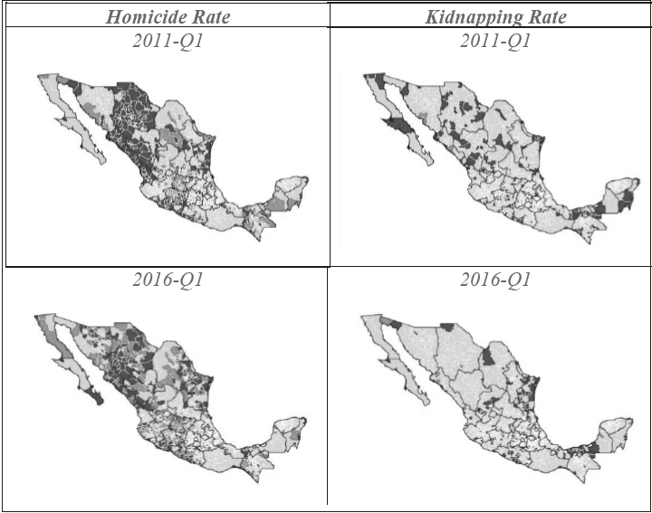
Note: Dark red represents two or more times the country average crime rate, red represents above the country average crime rate, but less than two times such crime rate. Yellow refers to below the country average crime rate and white to zero crimes registered in that period.
Source: CONAPO, INEGI Mexican National Public Security Executive Office, Mexican Interior Ministry.
Figure 1 Homicide and Kidnapping Rates, Mexico 2011-Q1 - 2016-Q1
Furthermore, the state of Tamaulipas, located in the north-eastern part of the country, shows a similarly high concentration of homicides. These dark areas on the map show that homicide rates in those places are twice as higher than the average rate in the country. When homicide rates are compared between 2011 and 2016 maps, 2016 homicides are still concentrated in the same states as in 2011, but with less intensity and were dispersed to other states such as Nuevo León and Baja California Sur. Also in both maps homicides are concentrated in the northern part of the country.
Figure 1 shows that in 2011 kidnapping rates were widely distributed across the country, but slightly more concentrated in the north. The yellow areas represent places where kidnapping rates were below the country average for that period. Then, in 2016, there are few municipalities with values two or more times higher than the country average. It is worth noting that Tamaulipas show the highest kidnapping rates in the country.
Regarding the use of official public crime data, Guerrero-Gutiérrez (2011) recognizes that an analysis based exclusively on official crime figures poses several shortcomings. These figures are usually published in comprehensive databases only after a long delay; moreover, the figures account exclusively for crimes reported to the authorities. Given Mexico’s law enforcement institutions’ reputation for low performance and pervasive corruption, many citizens choose not to report crimes. Moreover, fear of retaliation from criminal organizations may increasingly prevent victims from filing reports. Due to the uneven performance of law enforcement institutions as well as uneven criminal organization presence throughout the country, these factors may also bias cross-sectional analyses.
Also according to Soares (2004), the fraction of the total number of crimes reported to the police varies widely across countries and across different types of crimes. Reported crimes are likely to suffer from measurement error, which thereby introduces a source of bias.
Similarly, Magaloni et al. (2017) point out this matter for Mexico, arguing that government data might suffer bias from underestimation of case misclassification. In fact, for the crime incidents reported to local public attorney offices and victimization surveys in 2011 the authors estimate that underreporting bias is as high as 87.2% for common crime and 93.2% for extortion.
Additionally, for Mexico, González Andrade (2014) mentions that the underestimation of crimes is generated by victims who do not report the crime to the authorities or the authorities have not started a preliminary investigation.
While we recognize these limitations, and criminal prosecution and quantification is a complex problem, we use these datasets as our first source of information in keeping with other previous works in this same line of research.
Other variables
Other control variables included in our model are the alternative wage and exchange rate measured in real terms. The alternative wage was is a weighted average of all wages outside the considered locality. Wages are exclusively for the formal sector obtained from INEGI, capturing data from IMSS (Mexican Social Security Institution). The quarterly exchange rate is the average for the analyzed period as reported by the Banco de México website.
The state control variables include a proxy for the real state GDP dynamics variable, real direct foreign investment (FDI), average state education level, and state population. The quarterly indicator for State Economic Activity (ITAEE, 2008=100), available from INEGI, is useful for measuring economic conditions as a proxy for GDP. Following Cabral et al. (2015), we include new FDI reported by the Mexican Ministry of Economy website and available at the state level on a quarterly basis. The average number of school years completed for each state’s labor force, reported by the Ministry of Public Education (SEP), is also included following Partridge and Rickman (2005) and Mollick and Cabral (2015). State population comes from the National Council of Demographic Planning (CONAPO).
Finally, economic activity in Mexico differs greatly across the country’s geographic regions. Cuevas et al. (2002), Delajara (2012), and Fullerton Jr. (2001) find that economic performance in northern Mexico is more correlated with US economic activity than with that of southern and central Mexico. In addition, NAFTA has brought Mexico more economic independence between regions and a reduction in the importance of Mexico City (Rodríguez-Pose and Sánchez-Reaza, 2005). To account for these, we add dummy variables quantify fixed factors (north, center and south) and consider the proximity to the US (border).
IV. Results
Unitary changes in crime rate
Our unit of analysis is a locality, defined by metropolitan and non-metropolitan areas in each state in Mexico, i.e. 61 localities in total; we follow employment, crime rates and other variables for each locality quarterly from 2011 to 2016. The selection of state level metropolitan and non-metropolitan areas was in line with previous literature conducted for Mexico and is selected to maximize the information and variance we can extract from the statistics on crime and employment.
The models are estimated in logarithms for most of the control variables, except crime rates. Therefore, the parameters measure elasticities for most of the control variables, whereas the crime rate estimated parameter should be considered as a semi-elasticity.
In each model, we have employment by locality and firm size aggregators, and use the traditional explanatory variables and the different crime rates variable. The model estimations first include all localities (whole country), and are then divided into metropolitan and non-metropolitan, and the dependent variable total firm employment is broken down into firm employment, according to the number of employees per firm.
Endogeneity of crime rates at the local level in a given time period represents one of the biggest challenges for the correct identification of its effect on labor employment. To solve this issue, we followed a two-stage Instrumental Variable (IV) approach where we build a contemporary crime rate (kidnapping and homicide) instrument using its lagged value and the set of exogenous independent variables. Our selection of an instrument is consistent with other works, such as Grossman (1982), Hanson’s (2001) and more recently Coronado and Saucedo (2018).
Fisher (2010) describes Wooldridge’s (1995) alternative endogeneity test, suggested for testing endogeneity of an explanatory variable when using two-stage least squares with robust error model estimation. This test provides both the endogeneity test related to the key hypothesis variable (in our case contemporary crime rates), and provides the properties of the instrument as measured by the R-square values of the first stage regression and the joint F-test of the two equations.
We proceed to estimate Wooldridge’s tests on crime for each model analyzed and decompose the models at aggregate employment, metropolitan areas, and non-metropolitan areas. We report OLS and IV estimations of different versions of equation (1), identifying the effect of homicide and kidnapping rates in Tables 4 and 5, respectively. It is worth noticing that when we analyze total employment, Wooldridge’s test suggests that there is consistent evidence of crime rate endogeneity for both homicide and kidnapping. However, our instrument regression selection provides a valid measure, as shown in both Tables 4 and 5, with adjusted R-square values of first-stage regression of 0.8833 and 0.6102 for homicide and kidnapping, respectively, and joint model F-test with high significance p-values in all cases.
When we open our analysis by metropolitan and non-metropolitan areas, the results suggest endogeneity in the contemporary crime rate, except for homicide in non-metropolitan areas. We followed the same approach instrumenting crime with its lagged value and other control variables, which resulted in a valid instrument, as shown in Tables 4 and 5. For the rest of our analysis, we report the IV model results as the joint F-tests of the two-stage model suggest there is no loss of generality in using this approach, and it provides a direct comparison with the other cases.
Results in Table 3 indicate that no matter which model is used, the homicide rates have a statistically robust negative effect on total firm employment at a country level, but also in metropolitan and non-metropolitan areas. Estimations show that a one-unit increase in homicide reduces total firm employment between 0.05 to 0.15% in all localities. Nevertheless, when the analysis is focused on metropolitan and non-metropolitan areas separately, the IV estimation implies that an increase of 1 unit in homicide would lead to a loss in total firm employment of 0.15% and 0.22%, respectively.
Table 3 Employment and homicide rates Crime rate semi-elasticities by total, metropolitan and non-metropolitan areas: Mexico 2011-2016
| Independent Variable | Total Employment | Metropolitan Areas Employment | Non-Metropolitan Areas Employment | |||
|---|---|---|---|---|---|---|
| OLS | IV | OLS | IV | OLS | IV | |
| Homicide Rate in Locality | -0.0006* | -0.0015*** | -0.0005 | -0.0016** | -0.0017** | -0.0022** |
| (offenses per 100 000s inhabitants) | [0.0003] | [0.0005] | [0.0003] | [0.0006] | [0.0007] | [0.0009] |
| Real GDP (in Logs) | 0.0854*** | 0.0894*** | 0.0096 | 0.0058 | 0.1577*** | 0.1681*** |
| [0.0271] | [0.0272] | [0.0313] | [0.0321] | [0.0414] | [0.0420] | |
| Total Population (in Logs) | 0.7746*** | 0.7608*** | 0.8456*** | 0.8268*** | 0.9203*** | 0.9334*** |
| [0.0627] | [0.0685] | [0.0671] | [0.0732] | [0.1632] | [0.1864] | |
| Real Exchange Rate (in Logs) | 0.2073*** | 0.2127*** | 0.2068*** | 0.2033*** | 0.2017*** | 0.2192*** |
| [0.0342] | [0.0369] | [0.0385] | [0.0418] | [0.0545] | [0.0587] | |
| Total Foreign Direct Investment in Locality (in Logs) | 0.0002 | 0.0004 | 0.0002 | 0.0003 | 0.0081 | 0.0091 |
| [0.0011] | [0.0012] | [0.0007] | [0.0008] | [0.0176] | [0.0174] | |
| Average Education Years (in Logs) | -0.011 | 0.011 | 0.0803*** | -0.0597** | 0.0459 | 0.0709* |
| [0.0252] | [0.0261] | [0.0260] | [0.0284] | [0.0408] | [0.0421] | |
| Average Real Wage (in Logs) | -0.0894 | -0.0737 | -0.0791 | -0.0704 | -0.088 | -0.0667 |
| [0.0559] | [0.0583] | [0.0606] | [0.0658] | [0.0978] | [0.1001] | |
| Alternative Real Wage to Current Locality (in Logs) | 0.4587*** | 0.4556*** | 0.3169*** | 0.3172*** | 0.6255*** | 0.6260*** |
| [0.1028] | [0.1040] | [0.1101] | [0.1123] | [0.1705] | [0.1722] | |
| Border (Yes =1) | 0.0004*** | 0.0004*** | 0.0004*** | 0.0004*** | 0.1149** | 0.1465** |
| [0.0000] | [0.0000] | [0.0000] | [0.0000] | [0.0564] | [0.0606] | |
| North (Yes =1) | -0.8489*** | 0.2398*** | -0.5497** | -0.7923*** | -0.2589 | 0.1135 |
| [0.2995] | [0.0792] | [0.2476] | [0.2558] | [0.3540] | [0.1134] | |
| South (Yes =1) | 0.3958*** | 0.4300*** | -0.7175** | -0.5424** | 0.2268*** | 0.1623 |
| [0.0951] | [0.1039] | [0.3036] | [0.2452] | [0.0710] | [0.3218] | |
| Locality is SMA (Yes=1) | 0.8303*** | 0.8826*** | ||||
| [0.1947] | [0.2107] | |||||
| Constant | -2.4842* | -2.5209* | -0.4236 | -0.0932 | -6.9320** | -7.5968** |
| [1.2959] | [1.3434] | [1.5530] | [1.6324] | [2.9138] | [3.2103] | |
| Fixed Effect: Time | Yes | Yes | Yes | Yes | Yes | Yes |
| Fixed Effect: Locality | Yes | Yes | Yes | Yes | Yes | Yes |
| R-Squared | 0.9987 | 0.9987 | 0.9992 | 0.9993 | 0.9978 | 0.9978 |
| Adj. R-Squared | 0.9986 | 0.9986 | 0.9992 | 0.9992 | 0.9976 | 0.9977 |
| Sample size: n | 1280 | 1220 | 650 | 620 | 630 | 600 |
| Instrument hypothesis statistics7 | ||||||
| Robust score test (Chi-squared): | 6.98739*** | 5.36467*** | 1.63032 | |||
| Robust score test (p-value): | 0.0082 | 0.0205 | 0.2017 | |||
| Robust regression test (F): | 6.39373*** | 5.06564*** | 1.53901 | |||
| Robust regression test (p-value): | 0.0116 | 0.0248 | 0.2153 | |||
| First-stage instrument regression statistics8 | ||||||
| R-squared | 0.8904 | 0.8879 | 0.8889 | |||
| R-squared adjusted | 0.8833 | 0.8794 | 0.8804 | |||
| R-squared partial | 0.3947 | 0.3232 | 0.5673 | |||
| Joint model (F-test) | 91.1658*** | 42.2294*** | 246.686*** | |||
| Joint model (p-value) | 0 | 0 | 0 | |||
Notes:
1) The reported estimations on crime rate show a semi-elasticity impact on natural logarithms: a coefficient of X means that a unitary increase in crime rate induces an effect on the employment of exp(X)-1 over its current level. For example, an increase in crime offenses from 10/100,000 to 20/100,000 is equivalent to a measured change of 20 units. An estimated coefficient reported of -0.0015 indicates that an increment in 20 units on the crime rate would lead to a decrease in employment of 0.30% derived from this change.
2) Each model includes fixed effects control variables by locality and time; estimated coefficients in these items are not reported in this table.
3) The threshold level indicators for statistical significance (p-values) are: [*] p<0.10, [**] p<0.05, [***] p<0.01.
4) Instrument variables model specification uses the first lag of the crime rate and all the additional controls in the model including the fixed effects by locality and time.
5) The standard error for each coefficient is reported in parentheses.
6) Regional fixed-effect variables (North - Center - South), based on Chiquiar (2008).
7) Wooldridge’s (1995) robust score test and a robust regression-based test are reported; tests are performed to determine whether endogenous regressors in the model are in fact exogenous if the test statistic is significant, then the variables being tested must be treated as endogenous.
8) Reports various statistics that measure the relevance of the excluded exogenous variables. By default, whether the equation has one or more than one endogenous regressor determines which statistics are reported.
Source: Own estimations using CONAPO (2016) and INEGI (2011-2016).
Results also indicate that the alternative wage has a positive effect on state employment. One of the potential reasons for this is that employment data reported in this model come from ENOE, while wages included in the regression come from a government database, which only captures wages in the formal sector.
The real exchange rate, has a positive and statistically significant result in all models, reflecting Mexico’s greater attractiveness to foreign investment and increase in exports; these results are in line with authors such as Faria and León-Ledesma (2005), Hua (2007) and Alexandre et al. (2010).
Real aggregate market dynamics (ITAEE) is positive and directly correlated. Results are consistent in all localities and in non-metropolitan areas, as in Gosh (2009), Chiang, Tao and Wong (2015), and Klinger and Weber (2015).
The new FDI variable has a positive and statistically significant effect on employment only in non-metropolitan areas. Literature that supports this positive correlation for the Mexican economy is Mendoza J. (2011), the positive correlation between FDI is with high-skilled employment in the manufacturing industry, but not with all employment in this sector.
In addition, the fixed effects included in the model are statistically significant and indicate the existence of unobserved heterogeneity across geographic regions in the country.
Table 4 Employment and kidnap rates Crime rate semi-elasticities by total, metropolitan and non-metropolitan areas: Mexico 2011-2016
| Independent Variable | Total Employment | Metropolitan Areas Employment | Non-Metropolitan Areas Employment | |||
|---|---|---|---|---|---|---|
| OLS | IV | OLS | IV | OLS | IV | |
| Kidnap Rate in Locality (offenses per 100 000s inhabitants) | -0.0038* | -0.0366** | -0.0065*** | -0.0345** | -0.0067 | -0.1084*** |
| [0.0021] | [0.0154] | [0.0022] | [0.0158] | [0.0075] | [0.0404] | |
| Real GDP (in Logs) | 0.0853*** | 0.0811*** | 0.0096 | 0.0071 | 0.1558*** | 0.1191** |
| [0.0272] | [0.0293] | [0.0310] | [0.0346] | [0.0422] | [0.0509] | |
| Total Population (in Logs) | 0.7770*** | 0.7228*** | 0.8575*** | 0.8586*** | 0.8636*** | 0.5398** |
| [0.0636] | [0.0883] | [0.0687] | [0.0963] | [0.1701] | [0.2581] | |
| Real Exchange Rate (in Logs) | 0.2044*** | 0.2030*** | 0.2022*** | 0.1858*** | 0.1998*** | 0.2193*** |
| [0.0341] | [0.0388] | [0.0377] | [0.0444] | [0.0545] | [0.0652] | |
| Total Foreign Direct Investment in Locality (in Logs) | 0.0003 | 0.001 | 0.0004 | 0.0012 | 0.0071 | 0.0098 |
| [0.0011] | [0.0016] | [0.0008] | [0.0013] | [0.0176] | [0.0185] | |
| Average Education Years (in Logs) | -0.0094 | 0.0222 | -0.0754*** | -0.0469 | 0.0557 | 0.0863** |
| [0.0251] | [0.0272] | [0.0248] | [0.0325] | [0.0406] | [0.0403] | |
| Average Real Wage (in Logs) | -0.091 | -0.0464 | -0.075 | -0.0287 | -0.0996 | -0.0539 |
| [0.0556] | [0.0656] | [0.0588] | [0.0790] | [0.0978] | [0.1119] | |
| Alternative Real Wage to Current Locality (in Logs) | 0.4572*** | 0.4151*** | 0.3172*** | 0.3097** | 0.6177*** | 0.4115** |
| [0.1028] | [0.1148] | [0.1090] | [0.1279] | [0.1713] | [0.2081] | |
| Border (Yes =1) | 0.0004*** | 0.0003*** | 0.0004*** | 0.0004*** | 0.0817 | -0.0003 |
| [0.0000] | [0.0001] | [0.0000] | [0.0001] | [0.0593] | [0.0851] | |
| North (Yes =1) | -0.8422*** | -1.0987*** | -0.6256** | -0.5007 | -0.3858 | -0.4447 |
| [0.3041] | [0.4110] | [0.2750] | [0.3080] | [0.3702] | [0.3091] | |
| South (Yes =1) | 0.3915*** | 0.3372** | -0.5909** | -0.5061 | 0.2111*** | -0.5783 |
| [0.0957] | [0.1499] | [0.2831] | [0.3532] | [0.0722] | [0.4592] | |
| Locality is SMA (Yes=1) | 0.8253*** | 1.0069*** | ||||
| [0.1977] | [0.2721] | |||||
| Constant | -2.4918* | -1.7514 | -0.6376 | -0.7967 | -5.9405* | 0.3662 |
| [1.3072] | [1.6513] | [1.5780] | [2.1090] | [3.0358] | [4.7289] | |
| Fixed Effect: Time | Yes | Yes | Yes | Yes | Yes | Yes |
| Fixed Effect: Locality | Yes | Yes | Yes | Yes | Yes | Yes |
| R-Squared | 0.9987 | 0.9985 | 0.9993 | 0.999 | 0.9977 | 0.9971 |
| Adj. R-Squared | 0.9986 | 0.9984 | 0.9992 | 0.9989 | 0.9976 | 0.9969 |
| Sample size: n | 1280 | 1220 | 650 | 620 | 630 | 600 |
| Instrument hypothesis statistics6 | ||||||
| Robust score test (Chi-squared): | 5.92527*** | 3.48505* | 8.45948*** | |||
| Robust score test (p-value): | 0.0149 | 0.0619 | 0.0036 | |||
| Robust regression test (F): | 5.84268*** | 3.33505 | 10.1487*** | |||
| Robust regression test (p-value): | 0.0158 | 0.0683* | 0.0015 | |||
| First-stage instrument regression statistics7 | ||||||
| R-squared | 0.6338 | 0.6212 | 0.7031 | |||
| R-squared adjusted | 0.6102 | 0.5925 | 0.6804 | |||
| R-squared partial | 0.032 | 0.0245 | 0.0583 | |||
| Joint model (F-test) | 10.2676*** | 5.52175*** | 17.8599*** | |||
| Joint model (p-value) | 0 | 0.0042 | 0 | |||
Notes:
1) The reported estimations on crime rate show a semi-elasticity impact on natural logarithms: a coefficient of X means that a unitary increase in crime rate induces an effect on the employment of exp(X)-1 over its current level. For example, an increase in crime offenses from 10/100,000 to 20/100,000 is equivalent to a measured change of 20 units. An estimated coefficient reported of -0.0015 indicates that an increment in 20 units on the crime rate would lead to a decrease in employment of 0.30% derived from this change.
2) Each model includes fixed effects control variables by locality and time; estimated coefficients in these items are not reported in this table.
3) The threshold level indicators for statistical significance (p-values) are: [*] p<0.10, [**] p<0.05, [***] p<0.01,.
4) Instrument variables model specification uses the first lag of the crime rate and all the additional controls in the model including the fixed effects by locality and time.
5) The standard error for each coefficient is reported in parentheses.
6) Regional fixed-effect variables (North-Center-South) based on Chiquiar (2008).
7) Wooldridge’s (1995) robust score test and a robust regression-based test are reported; tests are performed to determine whether endogenous regressors in the model are in fact exogenous if the test statistic is significant, then the variables being tested must be treated as endogenous.
8) Reports various statistics that measure the relevance of the excluded exogenous variables. By default, whether the equation has one or more than one endogenous regressor determines which statistics are reported.
Source: Own estimations using CONAPO (2016) and INEGI (2011-2016)
Table 4 follows table 3 regarding the independent variables, but using kidnapping as the main dependent variable. Estimates show that kidnapping has a negative and statistically significant effect on total firm employment when all localities are analyzed together. A one-unit increase in the kidnapping rate decreases total employment between 0.36% and 3.45%. For metropolitan and non-metropolitan areas, the impact of an increase in 1 unit in the kidnaping rate reduces employment by 3.17% and 10.84%, respectively.
Our purpose is to analyze not only the effect of homicides and kidnappings on all firm employment, in metropolitan and non-metropolitan areas, but also the effect of such crimes in different firm sizes. Each of the following regressions has the same independent variables as in previous tables but the dependent variable corresponds to self-employment and employment in micro, small, medium and large firms in all localities, as well as in metropolitan and non-metropolitan areas4. All regressions on Table 5 include locality and time fixed-effect control variables.
Table 5 The effect of homicides and kidnappings on employment Crime rate semi-elasticities by locality and firm size: Mexico 2011-2016
| Crime Rate | Locality Aggregation | All Localities | Metropolitan Areas | Non-Metropolitan Areas | |||||||||
| Firm Size\ Method | OLS | IV | OLS | IV | OLS | IV | |||||||
| Homicide Rate | All Firms | -0.0006 | [a] | -0.0015 | [c] | -0.0005 | -0.0016 | [b] | -0.0017 | [b] | -0.0022 | [b] | |
| (0.0003) | (0.0005) | (0.0003) | (0.0006) | (0.0007) | (0.0009) | ||||||||
| Self-employed | 0.0003 | -0.0018 | -0.0001 | -0.0029 | [b] | 0.0016 | 0.0016 | ||||||
| (0.0006) | (0.0011) | (0.0007) | (0.0015) | (0.0012) | (0.0017) | ||||||||
| Micro | -0.0003 | -0.0012 | [a] | -0.0003 | -0.0014 | [a] | -0.0004 | -0.0005 | |||||
| (0.0004) | (0.0007) | (0.0004) | (0.0008) | (0.0010) | (0.0013) | ||||||||
| Small | -0.0014 | [b] | -0.0023 | [b] | -0.0008 | -0.0010 | -0.0035 | [b] | -0.0051 | [b] | |||
| (0.0007) | (0.0010) | (0.0007) | (0.0011) | (0.0014) | (0.0020) | ||||||||
| Medium | 0.0004 | 0.0011 | -0.0008 | -0.0012 | 0.0010 | 0.0021 | |||||||
| (0.0010) | (0.0016) | (0.0008) | (0.0017) | (0.0028) | (0.0032) | ||||||||
| Large | 0.0014 | 0.0026 | -0.0000 | -0.0003 | -0.0018 | -0.0013 | |||||||
| (0.0014) | (0.0024) | (0.0014) | (0.0027) | (0.0032) | (0.0043) | ||||||||
| Kidnap Rate | All Firms | -0.0038 | [a] | -0.0366 | [b] | -0.0065 | [c] | -0.0345 | [b] | -0.0067 | -0.1084 | [c] | |
| (0.0021) | (0.0154) | (0.0022) | (0.0158) | (0.0075) | (0.0404) | ||||||||
| Self-employed | -0.0111 | [b] | -0.0433 | -0.0100 | [b] | -0.0578 | [a] | -0.0085 | 0.0351 | ||||
| (0.0046) | (0.0288) | (0.0050) | (0.0341) | (0.0132) | (0.0630) | ||||||||
| Micro | -0.0040 | -0.0233 | -0.0069 | [c] | -0.0168 | -0.0024 | -0.0876 | ||||||
| (0.0026) | (0.0179) | (0.0027) | (0.0190) | (0.0114) | (0.0549) | ||||||||
| Small | -0.0028 | -0.0628 | [b] | 0.0001 | -0.0310 | -0.0270 | -0.1761 | [b] | |||||
| (0.0046) | (0.0295) | (0.0045) | (0.0279) | (0.0192) | (0.0841) | ||||||||
| Medium | 0.0057 | 0.0263 | -0.0020 | -0.0458 | -0.0116 | 0.1010 | |||||||
| (0.0066) | (0.0411) | (0.0062) | (0.0466) | (0.0301) | (0.1232) | ||||||||
| Large | 0.0042 | 0.0638 | -0.0134 | -0.0268 | 0.0198 | -0.0177 | |||||||
| (0.0102) | (0.0636) | (0.0095) | (0.0674) | (0.0407) | (0.1642) | ||||||||
Source: Own estimations using CONAPO (2016) and INEGI (2011-2016).
When firm employment is divided according to work size, the effects of homicide rates on employment are heterogeneous across firm size. On the one hand, findings indicate that when the homicide rate increases by 1 unit, in all localities self-employment, micro and small firm employment drop by 0.12%, 0.23%, and 0.23%, respectively. On the other hand, results in metropolitan areas show that when the homicide rate increases by 1 unit, self-employment decreases by 0.29% and micro firm employment drops by 0.14%. Results also indicate that changes in the homicide rate do not have a statistically significant impact on the employment rate of small, medium and large firms in metropolitan areas. In the case of non-metropolitan areas, estimations show that employment in small firms decreases by 0.51%, whereas all other employment by firm size is not statistically significant.
Regarding kidnapping rate, results indicate that when firm employment is divided according to the number of employees, firms employment responds more sharply to increases in the kidnapping rate than to a similar increase in the homicide rate.
Using IV estimations, results for all localities indicate that when there is a 1-unit increase in the kidnapping rate, small firm employment decreases by 6.82%. In metropolitan areas, the unitary increase in the kidnapping rate would lead to a decrease of 4.99% in self-employment; all these results support BenYishay and Pearlman (2013) findings. Finally, for non-metropolitan areas, an increase in one unit of this offense induces a 17.61% employment loss in small firms. These large increases due to kidnapping are related to the low probability of a simultaneous kidnapping unitary increase along all the localities given the current variance in each state and locality. Theory dictates that self-employment or small firms are more reactive than medium or large firms when violence increases, as supported by evidence in Amin (2009).
Our results on medium and large firms show employment on these firms’ size do not respond to crime rates changes, both for kidnap and homicide. This result is consistent previous research that demonstrates large firms have huge investments in fixed capital and other important costs, which makes it difficult for them to respond elastically when violence increases, in comparison to self-employed or small firms. For instance, Granovetter (1973) and more recently Brouwer et al. (2004) find that firms’ mobility incentives decrease with the size of the firm. In addition, McCann (2001) mentions that relocation costs may be quite significant as firms need to consider, among other factors, the cost of the real-estate site search and acquisition, dismantling, moving and reconstruction of existing facilities, and hiring and training new employees.
Kuratko et al. (2000) mention that small business are 35 times more likely to suffer from business crime than larger firms.
Finally, Perrone (2000), in a study for small firms in Australia, finds that certain occupational risks, such as working with the public, working in isolation, working late at night or in the early hours of the morning, being involved in the exchange of money, increase the vulnerability of small firms.
The results of this research are in line with previous literature capturing not only the effect of homicides and kidnappings on total firm employment in Mexico, but also identifying the relative vulnerability of smaller firms to crime.
Employment losses
Our next exercise considers estimating the effect of an increase of 1 standard deviation (SD) in the relevant crime rate by locality. Under normality of a random variable, approximately 68% of its total values are within one standard deviation (higher or lower) from the mean. Therefore, if the crime rate is treated as an exogenous variable, then the range μ ± σ represents where almost 70% where its values occur.
Estimates in Table 6 provide more intuitive results about the effect of different crimes on firm employment. Such numbers are obtained from the homicide and kidnapping semi-elasticities obtained previously. The estimation is performed for each locality and state, 61 in total, and for each type of employment according to firm size and are presented in an average of the percentage point losses in employment, for all localities, metropolitan, and non-metropolitan areas, and across firm sizes.
Table 6 The effect of homicides and kidnappings on employment by firm size Average employment rate losses for an increase in one standard deviation in relevant crime rate by locality and firm size Mexico 2011-2016
| Crime Rate | Locality Aggregation / Firm Size | Metropolitan Areas | Non-Metropolitan Areas | All Localities | |||
|---|---|---|---|---|---|---|---|
| Homicide Rate | Self-employed | -1.07% | 0.31% | -0.74% | |||
| Micro | -0.52% | ** | -0.10% | -0.49% | * | ||
| Small | -0.37% | * | -1.00% | ** | -0.94% | ** | |
| Medium | -0.44% | 0.41% | 0.45% | ||||
| Large | -0.11% | -0.25% | 1.06% | ||||
| All Firms | -0.59% | ** | -0.43% | ** | -0.61% | *** | |
| Kidnap Rate | Self-employed | -2.34% | * | 0.54% | -1.55% | ||
| Micro | -0.68% | -1.34% | -0.83% | ||||
| Small | -1.25% | -2.69% | ** | -2.24% | ** | ||
| Medium | -1.85% | 1.54% | 0.94% | ||||
| Large | -1.08% | -0.63% | 2.28% | ||||
| All Firms | -1.40% | *** | -1.66% | *** | -1.31% | ** | |
Notes:
1) The table shows the estimated average on the rate on employment losses on average, given an increase of 1 unit in the standard deviation of the crime rate. Each standard deviation is calculated for each state by locality, and then using the coefficients in Table 4 for rate of employment effect decomposition.
2) Following the Mexican Ministry of Economy (Secretaría de Economía DOF 06/06/2006) the official definition for firm size conditional on the number of employees is: micro (1-10), small (11-50), medium (51-250) and large (250 and more workers).
3) Each model includes fixed effects control variables for locality and time. The estimated coefficients are not reported in this table.
4) IV model specification uses the first lag of the crime rate and all of the additional controls in the model including the fixed effects by locality and time.
5) The standard error for each coefficient is reported in parentheses.
6) The threshold level indicators for statistical significance (p-values) are: [*] p<0.10, [**] p<0.05, [***] p<0.01.
Source: Own estimations using CONAPO (2016) and INEGI (2011-2016).
Using the IV estimation and focusing on the statistically significant coefficients, our results show that an increase in one standard deviation in homicide reduces total employment for all localities by 0.61% and, when estimated by firm size, the employment losses are 0.89% in micro and 0.94% in small firms. The increase in one SD for homicide rates for metropolitan areas induces a reduction in total employment of around 0.59%, but estimations for the self-employment sector and for micro firms are statistically significant, with an average reduction in employment of 0.37% and 0.52%, respectively. Finally, for non-metropolitan areas, an increase in one SD for the homicide rate in each locality reduces total employment by 0.43%, but the effect is mainly on small firms, with a 1.00% reduction in employment for this sector.
On the other hand, IV estimates for the effect of kidnapping on employment is less significant across localities and firm size. In particular, IV estimations show that 1 SD increase in kidnaping crime rate for each locality reduces employment for all localities and all firms by 1.31%, while the effect between metropolitan and non-metropolitan areas is -1.40% and -1.66%, respectively. In this case, the effect for all localities is only significant in small firms, with a decrease of -2.24% in employment. For metropolitan areas, the effect is a reduction of 2.34% in self-employment, while non-metropolitan areas displayed a decrease of 2.69% in small firm employment.
For the second measure of job destruction due to crime, we use these percentage estimations in Table 6 and apply them to the latest employment observations, allowing us to estimate the number of employment losses.
Table 7 shows the point estimations of employment losses due to a one-SD increase in crime rate, divided by crime type, locality and firm size.
Using the IV estimation, we observe that an increase in one SD in the homicide rate in each locality reduces total employment by 560,705, while the reduction is around 256,969 jobs in metropolitan areas and 387,547 jobs in non-metropolitan areas. The estimation of employment losses due to this same increase in homicide crime rates for all localities is 106,307 in micro-firms and 78,532 in small-firms; 64,418 in micro-firms and 21,280 in small firms for metropolitan areas; while, for non-metropolitan areas, the job losses are significant for small firms, at approximately 31,152.
Table 7 The effect of homicides and kidnappings on employment by firm size Total employment losses for an increase in one standard deviation in relevant crime rate by locality and firm size Mexico 2011-2016
| Crime Rate | Locality Aggregation / Firm Size | Metropolitan Areas | Non-Metropolitan Areas | All Localities | |||
|---|---|---|---|---|---|---|---|
| Homicide Rate | Self-employed | -83,490 | 20,376 | -105,442 | |||
| Micro | -64,418 | ** | -9,380 | -106,307 | * | ||
| Small | -21,280 | * | -31,152 | ** | -78,521 | ** | |
| Medium | -19,083 | 6,631 | 24,744 | ||||
| Large | -3,703 | -5,620 | 51,511 | ||||
| All Firms | -181,988 | ** | -99,184 | ** | -319,542 | *** | |
| Kidnap Rate | Self-employed | -101,744 | * | 35,421 | -179,205 | ||
| Micro | -51,531 | -134,842 | -153,853 | ||||
| Small | -42,061 | -78,475 | ** | -140,461 | ** | ||
| Medium | -44,523 | 23,369 | 37,346 | ||||
| Large | -21,622 | -11,870 | 91,637 | ||||
| All Firms | -256,969 | *** | -387,547 | *** | -560,705 | ** | |
Notes:
1) The table shows the average estimated employment losses by locality and firm size type, given an increase of 1 unit in the time series standard deviation of the crime rate for each of the 61 localities. Each standard deviation is calculated by state and locality, and then the final effect is estimated using the coefficients in Table 4 for rate on employment effect decomposition at firm size and locality. The estimated rate of employment loss is applied on each of the relevant level of employment time series average on each locality and state.
2) Following the Mexican Ministry of Economy (Secretaría de Economía DOF 06/06/2006) the official definition for firm size conditional on the number of employees is: micro (1-10), small (11-50), medium (51-250) and large (250 and more workers).
3) Each model includes fixed effects control variables for locality and time. The estimated coefficients are not reported in this table.
4) IV model specification uses the first lag of the crime rate and all of the additional controls in the model including the fixed effects by locality and time.
5) The standard error for each coefficient is reported in parentheses.
6) The threshold level indicators for statistical significance (p-values) are: [*] p<0.10, [**] p<0.05, [***] p<0.01.
Source: Own estimations using CONAPO (2016) and INEGI (2011-2016).
Finally, an increase of one SD in kidnapping rates in each locality has a weaker significant effect on employment losses. In particular, the effect is a reduction in 101,744 job losses for the self-employed in metropolitan areas, and 78,475 jobs in small firms for non-metropolitan areas.
Our main conclusion of this section is, once we control for other relevant variables, employment in medium- and large-sized firms does not respond to crime rates, whereas employment in small, micro, and self-employed are relatively more responsive to increases in these felonies.
CONCLUSIONES
We analyzed the effect of homicides and kidnappings on self-employment, micro, small, medium and large firms in metropolitan and non-metropolitan areas in Mexico.
In our paper, we use an instrumental variable approach to correct the potential endogeneity of contemporary crime. Our results suggest that crime effects on job losses are quite diverse between metropolitan and non-metropolitan areas, and among different firm size employment. The estimations and results are robust and consistent across OLS and IV models. IV estimates also show robust results for all localities and for metropolitan and non-metropolitan areas.
We found that an increase in one unit in homicide crime rates reduces total employment by 0.15% in the country, and 0.15% and 0.22% in metropolitan and non-metropolitan areas, respectively. When firm employment is divided into firm categories, self-employment decreases by 0.11% in metropolitan areas. Similarly, when homicides increase by 2 units, micro-firm employment decreases by 0.11% in all localities and 0.13% in metropolitan areas, while the effect on non-metropolitan areas is not statistically significant. Lastly, a unitary increase in homicide crime rate decreases employment in small firms by 0.23% in all localities and 0.51% in non-metropolitan areas.
On the other hand, IV estimates show that a unitary increase in kidnapping rates reduces total firm employment by 0.36% in all localities, while non-metropolitan areas have a stronger effect on percentage points than their metropolitan peers. Results also show that regardless of the model implemented or geographic region analyzed, medium and large firm employment does not seem to respond to changes in the crime rate.
When we apply these point estimations to calculate the effect on job losses, assuming an increase of 1 SD in the homicide crime rate in each of the localities studied, our results imply a reduction in total employment by 319,542 jobs. When we expand our analysis by locality type, firm size and state, the reduction is around 181,988 jobs in metropolitan areas and 99,184 in non-metropolitan areas. On the other hand, a 1 SD increase in each locality for kidnapping crime rate induces a global reduction in employment of 140,461 in small firms, and when including locality and firm size, these results imply 101,744 job losses for self-employed in metropolitan areas and 78,475 jobs in small firms for non-metropolitan areas.
Results reported in this paper could shed some light on how homicides and kidnappings have affected employment in the self-employed, micro, small, medium and large firms in metropolitan and non-metropolitan areas across Mexico. These estimates can help to better understand the relevance of geographic location of firms, which could need higher police protection, and at the same time help, policymakers develop more efficient regional public policies focused on crime reduction. In particular, effective crime reduction within plausible values (for instance, 1 SD) might induce through efficient labor mark et al. location an increase in employment all over the country of up to 320 thousand new jobs, helping to reverse the negative consequences of the crime war over the last 20 years.

