Introduction

The realization that most biological phenomena are nonlinear systems occurring at different scales has represented a major scientific shift in all areas of biology. Most of these advances have occurred in the last 30 years thanks to new mathematical approaches and the development of large data sets readily accessible from internet. A nonlinear system is one that does not satisfy the superposition principle (f (x + y) = f (x) + f (y)), or one whose output is not directly proportional to its input, or one in which the sum of its parts is greater (or lesser) than the whole.

Most time we must deal with distributions of measures which are both smooth and well-behaved. In these cases, the distributions are described by well-known functions, they are differentiable, integrable, and continuous everywhere, except in an enumerable number of points. However, some time, nature shows up with quantities which cannot be described by smooth nor well behaved functions instead. These quantities, or measures, are, in general, distributed in a complex singular way (^{Mandelbrot 1998}). Singular distributions of physical and biological quantities may determine an infinite set of fractal dimensions each corresponding to the distribution of a given kind of singularity of the measure. In this case, not one but an infinity number of exponents are needed to describe each singularity, these exponents form a spectrum which is called the multifractal spectrum. These quantities are called multifractals if the multifractal spectrum is nontrivial. Fractal curves are known to be scale invariant, which means that the statistical properties of the signal remain invariant under scale transformations (^{Mandelbrot 1998}). In view of the heterogeneous (patchy) nature of the incidence time series of various childhood epidemics, we contend in this paper that a single exponent is not sufficient to characterize the complexity of epidemic dynamics, and that a multifractal approach may be necessary. In this work, we offer one example of how we can extract information about the scaling properties and the nonlinear character of a biological signal. We are interested in demonstrating that rubella epidemics follow a nonlinear dynamic and are more than a monofractal. To test the hypothesis that more than one scaling exponent are required to characterize epidemic dynamics, a continuous wavelet transform (CWT) and a multifractal analysis of the time series of rubella epidemics are performed. The article is organized as follows. First, we describe the biological signal followed by the mathematical background that will be used to analyze it. The main goal is to reveal hidden patterns from the observed dynamics of the monthly incidence of rubella in Mexico. By hidden patterns, we mean information that is neither visually apparent nor extractable with conventional methods of analysis. Such conventional techniques include the tacit assumption of a linear system or stationarity, estimation of means, standard deviation and other features of histograms.

Rubella epidemics

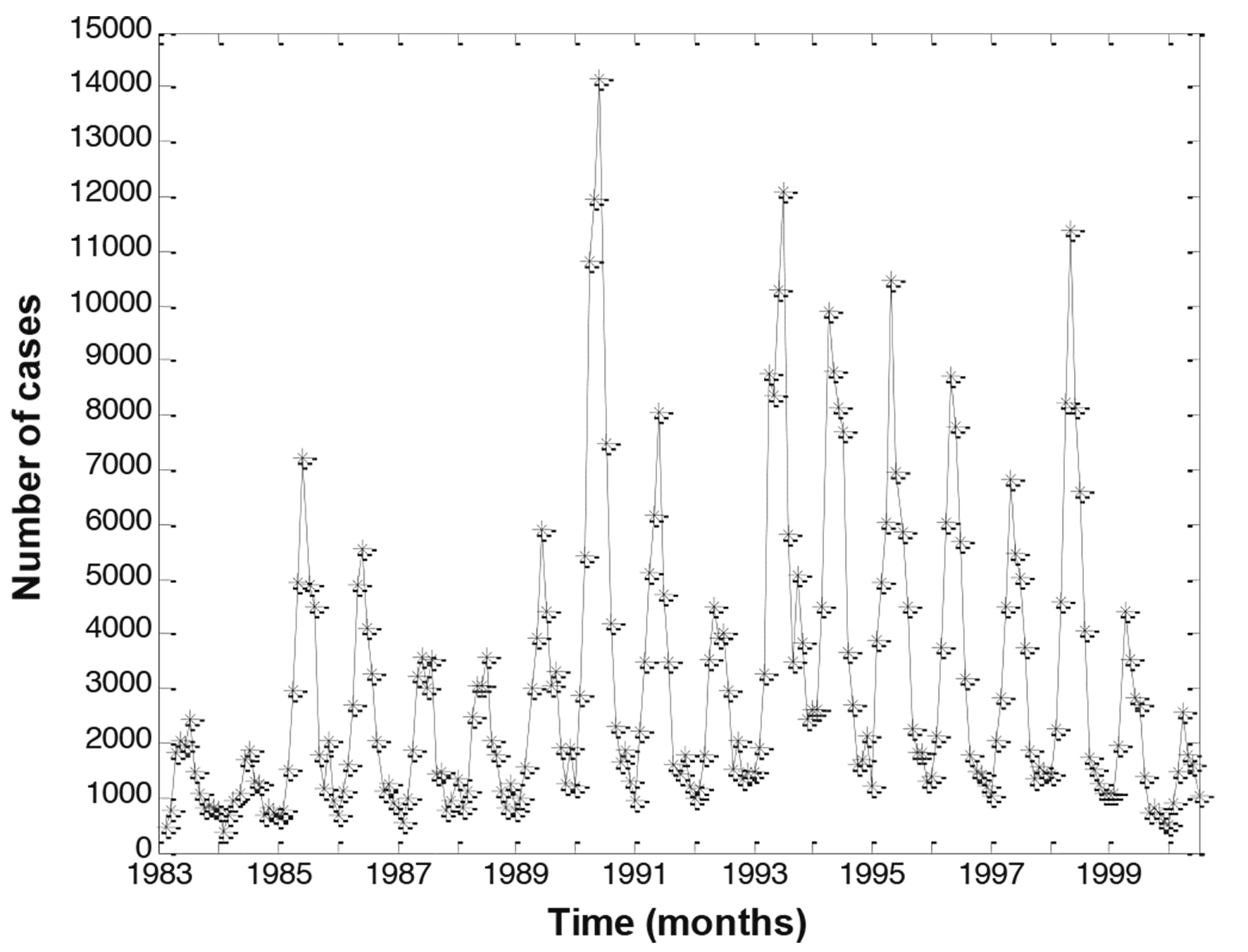
The monthly incidence of rubella in Mexico is shown in Figure 1. The characterization of the rubella epidemics in Mexico can be found elsewhere (^{José et al.,1992}). Note that there is an oscillatory behavior with seasonal annual cycles like several infectious diseases like influenza, measles, mumps, chickenpox (varicella), and poliomyelitis. It is also clear that the magnitude of the epidemic cycle of 1999 is the greatest. The main goal of vaccination against rubella infection is to prevent congenital rubella. After the year 2000, the rubella infection in Mexico started to decline until its virtually elimination around 2006. This success was mainly achieved be increasing the coverage of vaccination of young girls and boys. There are several cycles embedded in this time series. In particular, there is an inter-epidemic period every 4 years as observed by calculating the Fourier transform (not shown), which is not apparent by a simple visual inspection of the time series.

Source: Created by the authors.

Figure 1 Monthly incidence of rubella in Mexico 1983-2001.  

Wavelet transform

Unlike Fourier, wavelet transform (WT) is usually devoted to the analysis of non-stationary and nonlinear signals. Traditional approaches (such as the power spectrum and correlation analysis) are not suited for such non-stationary sequences, nor do they carry information stored in the Fourier phases which is crucial for determining nonlinear characteristics. Thus, there is no prerequisite over the stability of the frequency content along the signal analyzed. Conversely to Fourier, WT allows one to follow the temporal evolution of the spectrum of the frequencies contained in the signal. The shape of the WT-analyzing wavelet equation differs from the fixed sinusoidal shape of the Fourier transform and can be designed to better fit the shape of the analyzed signal, allowing a better quantitative measurement. Like Fourier or Laplace transforms, the continuous wavelet transform (CWT) is an integral transform. WT can be considered as a local Fourier analysis performed at different separated levels. A formal definition of the CWT is now given.

Definition of the wavelet transform

We introduce the one-dimensional continuous wavelet transform (CWT) and some of the basic mathematical results. We consider a function L ²(R, dt). We decompose this function S in terms of elementary functions obtained by dilations and translations of the real valued mother function Ψ(t). Let us define Ψ _a,b = a ^-1/2 Ψ((t - b)/a). The WT of s(t) is defined as (^{Daubechies 1994}):

where ••L2(R,   dt) is the scalar product in L ²(R, dt). Thus the WT is basically the scalar product of the function with the analyzing wavelet dilated by a and translated by b.

The analysis amounts to sliding a window of different weights (corresponding to different levels) containing the wavelet function all along the signal. The weights characterize a family member with a particular dilation factor. Thus the wavelet coefficients correspond to the scalar product of the given signal S with the wavelets Ψ _{a, b} (t) obtained by dilating (a) and translating (b) the analyzing wavelet Ψ(t). In other words, the WT T gives a serial list of coefficients called the wavelet coefficients and represents the evolution of the correlation between the signal S and the chosen wavelet at different levels of analysis (or different ranges of frequencies) all along the signal S.

The WT T is sometimes called a mathematical microscope or telescope because it allows the study of the properties of the signal on any chosen scale a. For high frequencies (small a), the Ψ functions have good localizations (being effectively non-zero only on small sub-intervals), so short-time regimes or high-frequency components can be detected by WT.

CWT of rubella epidemics

We have calculated the CWT using a broad range of orthonormal, compactly supported analyzing wavelets (^{Misiti et al. 2000}). We present results for the reverse biorthogonal wavelet pairs: rbioNr.Nd. The order is represented by Nd and Nr (d for decomposition and r for reconstruction). We chose this analyzing wavelet because the shape of both its reconstruction and decomposition wavelet functions (psi-scaling functions), resemble the short-term oscillatory behavior of the first differences of the monthly incidence of rubella in Mexico. Similar results were obtained using other wavelets such as Haar and coiflet 2 (not shown).

In Figure 2 the CWT of rubella incidence using as an analyzing wavelet the reverse biorthogonal spline with Nr = 1 and Nd = 3 (rbio1.3) is shown. Note that every year there are three rhombi of similar size throughout 64 scales indicating self-similar fractal behavior of the signal. It is also evident that there is a symmetrical pattern of the CWT over time. In particular, note that there are uninterrupted dark diagonal straight lines: some diagonals increase over time, from small scales to large scales, whereas other diagonals decrease over time, from large scales to small ones. The resulting pattern is that of several repetitive triangles consecutively formed over time. Some of these triangles have their bases at high frequencies (small scales), whereas in others their bases occur at very low frequencies (large scales). Note also that these triangles are part of the three rhombi formed every year, and of the rhombi formed every 4 and 6 years. Because the darker colors indicate the smallest values of the wavelet amplitudes, the dark diagonals represent the distribution of 61 quasi-fade-outs (small number of cases) of the original time-series over time and for all scales. The emerging successive and symmetrical triangles that arise from this distribution of darker diagonals constitute the skeleton of the whole pattern of the resulting WT. The transmission of rubella infection seems to be a multiplicative process, following a power-fractal scaling repelled from these dark diagonals. Each year there are bright vertical lines that cross all scales and that arise from the vertex of some of these triangles at very low frequencies.

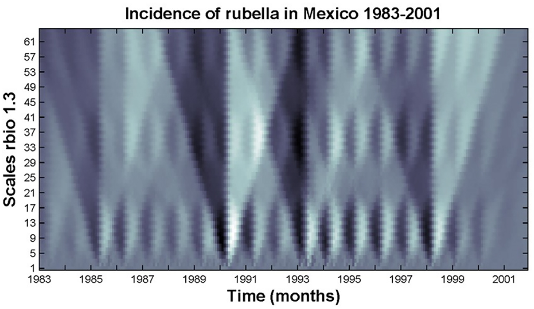
Note: The x-axis represents time (209 months) and the y-axis indicates the scale of the wavelet used (α = 1, 2, … , 64) with large scales (low frequency) at the top. The brighter colors indicate larger values of the wavelet amplitudes. The WA was performed with the reverse biorthogonal spline with Nr = 1 and Nd = 3 as an analyzing wavelet and it uncovers a hierarchical scale invariance quantitatively expressed by the stability of the scaling form. This wavelet decomposition reveals a self-similar fractal structure in the incidence of rubella every year, i.e. there are three rhombi of similar shape at different ranges of the scale. The CWT also unravels a repetitive pattern of successive triangles that are formed over time.

Source: Created by the authors.

Figure 2 Color-coded CWT of the incidence of rubella.  

Multifractals

The multifractal formalism is a statistical description that provides global information on the self-similarity properties of fractal objects (^{Sornette 2000}). A practical implementation of the method, consists first in covering the system of linear dimension L under study by a regular square array of some given mesh of size l. One then defines the measure of interest within the box. A simple fractal of dimension α is defined by the relation:

Simply put, a multifractal is a generalization in which α may change from point to point and is a local quantity. The standard method to test for multifractal properties consists in calculating the so-called moments of order q of the measure P _n defined by:

where n(l ) is the total number of non-empty boxes. If scaling holds, then one has

which defines the generalized dimension q. For instance, D ₀ corresponds to the capacity dimension; D ₁ and D ₂ are the information and correlation dimensions, respectively. In multifractal analysis, one can also determine the number N(l) of boxes having similar local scaling characterized by the same exponent α. As suming self-similar scaling,

Defining f(α) (the so-called multifractal singularity spectrum) as the fractal dimension of the set of singularities of strength α the sum (3) can then be rewritten as:

where J is the Jacobian of the transformation from the box index to its exponent α.

Comparing (6) with the definition (4), we find the general relation between a moment of order q and the singularity strength α, expressed mathematically as a Legendre transformation:

To obtain (7), we have used the fact that the Jacobian does not exhibit singular behavior for small l and thus does not contribute to the scaling law. Physically, expression (7) means that one set of boxes characterized by the same singularity α controls a given moment of order q.

Let us consider a geometrical support, where the quantity we are interested in is measured. Let L denote the actual linear size of the support and M the total value of the quantity on it. Now, let’s cover the support by boxes of size l such that, a << l << L, where a is the lattice constant, i.e., the microscopic size of the support. If m _i is the total amount of the quantity measured inside the ith non- empty box, we define the measure index, or Hölder exponent, α _i of this box by,

Selecting the boxes which correspond to the same Hölder exponent α we will have a subset of all boxes. This subset is a fractal with fractal dimension f(α) that is,

where N(α) is the number of boxes corresponding to a Hölder exponent α. If there exist a set of different Hölder exponents the measured will be a multifractal measure, hence its distribution shows a highly complex set of singularities. Alternatively, instead of the singularity spectrum, one can obtain a set of generalized dimensions D _q corresponding to the qth moment of the measure.

Again, if we cover the support with boxes of size l we have,

Actually, the generalized dimensions were introduced earlier, and it had been easier to computer it than the f(α) spectrum. The set of generalized dimensions characterize the nonuniformity of the measure, positive q accentuate denser regions and negative q accentuate rarer ones. When q = 0 we obtain the dimensions of the support, when q = 1 we have the information dimension. When both f(α) and D _q are smooth functions they are related by a Legendre transformation, actually, f(α) is the Legendre transform of τ(q) ≡ (q - 1) D _q . Although both formalisms, namely the f(α) and the D _q formalisms, are equivalent, the description of a multifractal measure is more natural by the f(α) spectrum. This is so because the singularity spectrum (f(α)) gives us an intuitive description of the interwoven sets, with differing singularity strengths α, whose Hausdorff dimension is f(α). To compute the singularity spectrum directly from data, we will apply the method developed by ^{Chhabra and Jensen (1989}) and ^{Chhabra et al. (1989)}. This method can directly determine the singularity spectrum f(α) from experimental data from systems where the underlying mechanisms are not well known.

The recipe of the Chhabra and Jensen method is the following. Given the experimental measure on the support, which has linear size L cover the support with boxes of linear size l such as in the equations (2) and (3). If m _i (l ) is the averaged value of the measure inside the ith box, construct the one-parameter family of normalized measures 𝜇(q) whose value in the ith box is,

The role of q is the same as in the generalized dimensions, q > 1 implies region for stronger singularities, q < 1 regions of weaker singularities, and q = 1 gives the original measure. The information dimensions of 𝜇(q) is,

and the average value of the singularity strength (or Hölder exponent) is,

These two expressions give us the singularity spectrum in terms of the q parameter.

Now we are ready to apply equations (11), (12), and (13) to our data. The support in our case is the period of observations, the measurements are the number of monthly number of rubella cases in Mexico during the period.

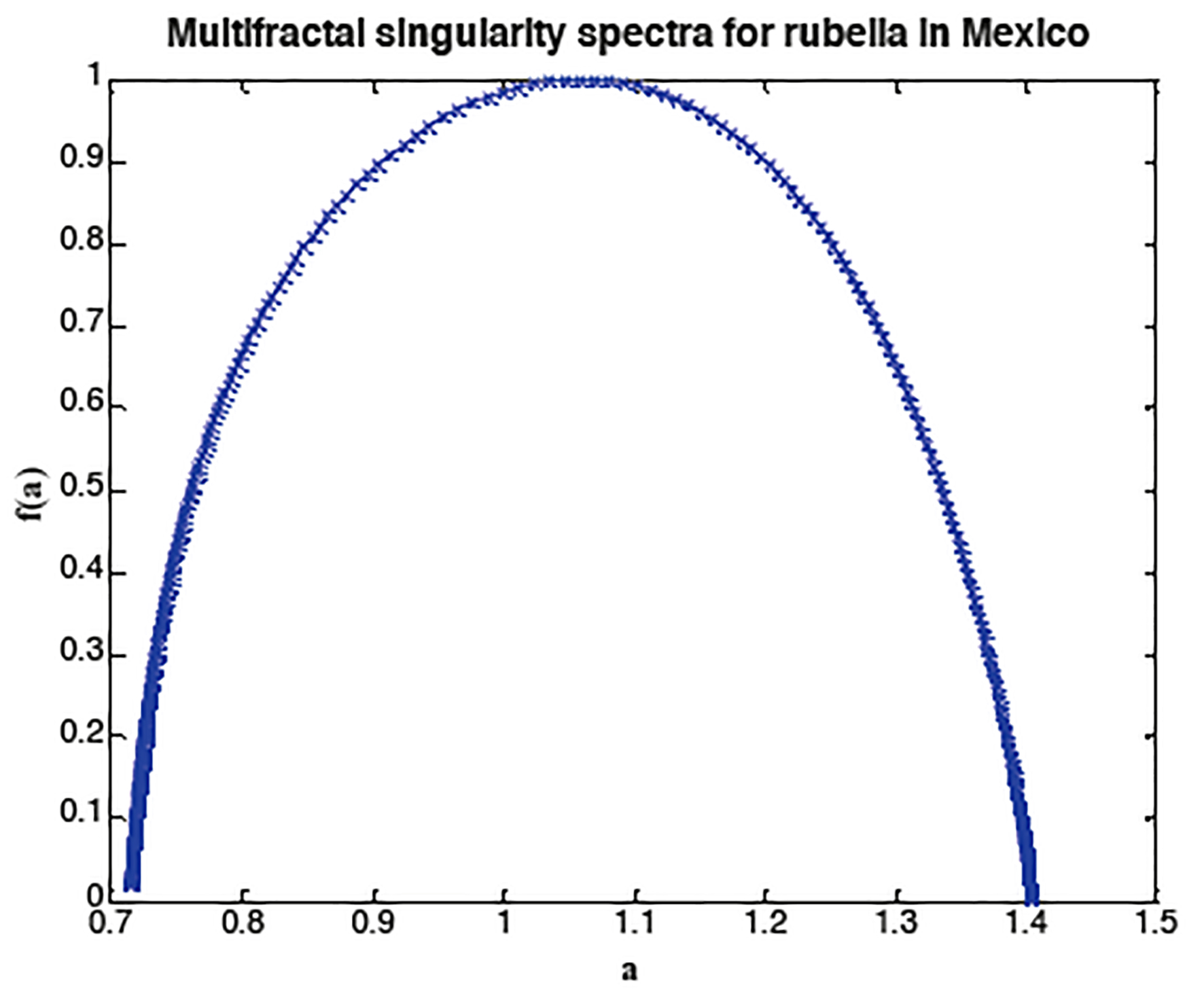
Multifractal spectra of rubella epidemics

The CWT of the epidemics of rubella suggested a multifractal dynamic. Therefore, we calculated the multifractal spectra of the rubella incidence in Mexico (Figure 3).

Source: Created by the authors.

Figure 3 The fractal singularity spectra versus the Hölder exponent.  

Conclusions

We have shown how to extract the scaling behavior of the monthly incidence of rubella infection. We have used the wavelet transform and the multifractal spectra of the time series. The signal is fractal every year, multifractal over time, and a symmetrical pattern emerges from the CWT.

All epidemiological models of infectious diseases consist of dividing the population into several compartments such as susceptibles, infected, and recovered (SIR models and variations of this). As far as we know, there are not mathematical epidemiological models that produce multifractal series of epidemiological phenomena. Fractional differential equations are needed to model this scaling pattern. We have illustrated that rubella epidemics display a symmetrical fractal annual pattern (self-similar) and multifractal dynamics. Symmetrical patterns in the epidemiology of rotavirus infection have also been found (^{José and Bishop 2003}). To characterize the complexity of epidemic dynamics, a multifractal approach is necessary, since several scaling exponents capture the dynamics at different scales.

The rapid changes in the time series are called singularities of the signal and their strength is measured by the crowding index α (Hölder exponent) (^{Struzik 2000}). The f(α) singularity spectrum provides a mathematically precise and natural intuitive description of the multifractal measure in terms of interwoven sets, with singularity strength α whose Hausdorff dimension is f(α) (^{Chhabra and Jensen 1989}).