nueva página del texto (beta)
 Inglés (pdf)
 Artículo en XML
 Referencias del artículo
 Enviar artículo por email
 Citado por SciELO
  Similares en
SciELO
Similares en
SciELO 
 Permalink
1. Introduction
This paper examines the relationship between domestic household migration and child labour in Mexico. In Mexico, 15 out of 100 people are child domestic migrants; this is an estimate of the population aged 5 to 17 years who resides in a location different from their birthplace. The Mexican Population Census estimates a rate of immigration of approximately 3.8 percent in 2000 and 2.9 percent in 2010, according to the 2018 Mexican National Survey of Demographic Dynamics (Encuesta Nacional de la Dinámica Demográfica, ENADID). There are several determinants of household decisions to migrate. Neoclassical economic theory has been the dominant framework for explaining internal migration in less developed countries (White and Lindstrom, 2005). People decide to migrate as a rational decision based on the maximum discounted lifetime earnings accounting for the moving costs for all household members (Mincer, 1978). Therefore, migration results from regional differences in income opportunities, which, in turn, depend on imbalances in the spatial distribution of factors of production (Dussault and Franceschini, 2006) and wage differentials (Harris and Todaro, 1970).
Migration is conceived as the movement of an individual from an area of origin to an area of destination, the essence of which is the change of habitual residence (Fussell and Massey, 2004). Internal migration is the movement of people between habitual residences within the geographical boundaries of a country (Rees, 2020). In this study, we analyse immigrant households and new resident households as equivalents because they face limited information compared to habitual household residents regarding where to look for a job and schools for their children, and they have limited support networks that help them (Edelblute and Altman, 2021). Because family members usually move together (DaVanzo, 1976; Van de Glind, 2010), we take the household as the unit of analysis. Following Patrinos and Psacharopoulos (1997), we assume that household migration and child labour choices are made within the child's current household.
Previous evidence suggests that the early inclusion of a child in child labour negatively affects children's current well-being and is detrimental to the expected future well-being (Li and Sekhri, 2020; Maya, 2021). On the other hand, child labour enhances cultural, social, family, and household living conditions (De Mesquita and de Farias, 2018). During migration assimilation, new resident households face income pressures that make them more likely to send children to work than habitual resident households (Rosati and Rossi, 2003). In addition, previous studies have suggested that migration makes children increasingly vulnerable to child labour and results in them being involved in the worst forms of labour, such as jobs with markedly longer hours or jobs with low wages (Edmonds and Shrestha, 2013; Immink and Payongayong, 1999).
In this paper, we define child labour as a person aged 5 to 17 years participating in any economic activity during the week preceding the interview (Edmonds, 2007). This paper aims to test whether children in new resident households (referred to as immigrants or migrants) have a greater probability of working than children living in nonimmigrant households in Mexico. One disadvantage to measuring migration and child labour effects is the limited information available, particularly about migration. In the present study, immigrant households are defined as those that declare being new residents during the last year. We use the 2013 Child Labour Module (Modulo de Trabajo Infantil, MTI), collected in the fourth quarter, to complement the labour survey of the 2013 National Survey of Occupation and Employment (Encuesta Nacional de Ocupación y Empleo, ENOE). Using these data gives us a better migration measure; the limitation is the outdated data. We inferred migration status from the new residents; we then compared the numbers of migrants per Mexican state with the population census. The resulting comparison provides evidence of a good migration proxy.
One of the issues in the study of migration when evaluating the differences between non- immigrant households and immigrant households is the selectivity of the latter (Aguayo-Téllez and Martínez-Navarro, 2013). The empirical strategy addresses the self-selective process in the household decision to migrate and its effect on child labour; there are two mixed effects on child labour decisions. First, the inverse correlation between child labour and education time (Bhalotra and Tzannatos, 2003). Second, the endogeneity in the migration process, usually the migrant population is not randomly selected, i.e., some individuals have skills and attribute that makes them more likely to migrate (Borjas, 1999). This paper models these two decisions using a bivariate probit model composed of two binary dependent variables. One is for the outcome of child labour, and the other is for household decision migration. First, we estimate child labour and recent household migration determinants separately. Then, we account for both equations to consider the unobserved factors. As a preview of our main results, we find statistically significant differences in child labour participation between children living in nonimmigrant households and children living in immigrant households. The latter has a greater probability of working. In addition, the results are consistent with previous evidence on child labour. Namely, the probability of working increases with age, child labour is more remarkable for boys than girls, and there is an inverse relationship between school attendance and child labour.
The rest of the paper is as follows. Section 2 presents a brief review of the literature on migrant children. Section 3 presents descriptive statistics about the children in the dataset to provide context. Section 4 introduces the empirical strategy and section 5 presents the results. Finally, section 6 concludes.
2. Literature Review
In most cases, migration offers new opportunities to households and their children, making it a survival solution for households in need. Several factors influence the decision to migrate, such as conflicts and natural disasters, domestic violence, household income, and the search for wellbeing for household members. Hence, migration can be a positive experience: it can provide people with a better life, increased job opportunities, an escape from immediate threats such as forced marriage, and access to education or better education (Hashim, 2005).
Additionally, migration may provide an opportunity to escape from existing divisions in the social order, allowing migrants to work with dignity and freedom at their destinations (Deshingkar and Akter, 2009). Unfortunately, migration makes children increasingly vulnerable to child labour (Patrinos and Psacharopoulos, 1997). Children from larger households are more likely to work because fewer resources must be shared among more household members. Another adverse effect is educational outcomes. In some cases, migrant students must repeat a grade, regardless of their age or learning needs, due to stringent school procedures and the absence of remedial classes to address students' learning deficits (Custodio and O'Loughlin, 2017; Guo et al., 2018). These students may have missed weeks or months of the school year while accompanying their parents to their destination when migration cycles begin (Coffey, 2013). Migration may cause children to forget what they have learned in school or prevent them from developing relationships with teachers and classmates to help them progress through school. Upon returning to their home villages, migrant children face multiple challenges, including learning difficulties that result from attendance disruptions (Gindling and Poggio, 2012).
Mexican evidence provides results on the effects of parental migration in the context of international migration. When the father migrates to the U.S., because of his absence, the short-run effects on his children's schooling and labour children reduce the number of hours they spend studying and their participation in schooling (Antman, 2011). Additionally, when a household member is a migrant, both boys and girls are less likely to complete high school and have a higher probability of entering the labour force (McKenzie and Rapoport, 2011). Children in migrant households complete significantly fewer schooling years (Hanson and Woodruff, 2003). In contrast to these results, a father's absence due to migration is likely to increase children's schooling because of remittances (Malone, 2007). In these cases, mothers are more likely to see education as one of the best uses of extra income abroad. Therefore, improvements in a child's educational attainment may be more likely when the father migrates, leaving the mother responsible for the use of remittances and the determination of resource allocations.
Children's birth order and household income level affect the allocation of time to attend school and child labour; older children have a lower probability of school attendance and higher labour participation than their siblings (Orraca, 2014). For children aged 5 to 11 years old, there is an inverse relationship between school attendance and child labour; the differences in labour participation are due to gender and higher labour participation in rural localities (Miranda-Juárez and Navarrete, 2016). However, none of these previous studies have explicitly studied the relationship between child labour and internal migration.
3. Data
This paper uses the 2013 MTI collected in the fourth quarter to complement the 2013 ENOE. We match the information of the population aged 12 to 17 years regarding child labour participation and school attendance with their household situations, such as their migration, labour, and employment characteristics (INEGI, 2013). Each sample household was interviewed five times at three-month intervals, and the sample was a rotating panel of five roughly equal groups, with a sample size of 121 116 households. Because only one randomly selected child in each household was interviewed, the final objective sample was 95 496 children. Appendix 2 presents more descriptive statistics for the sample.
We follow the definition of a child worker as a person aged from 5 to 17 years who performs any economic activity or has plans to do so (ILO, 2002). Economic activity is production for individual consumption, or any other action intending to produce or provide goods and services to the market. These activities may be paid or unpaid, and the activity could be in rural or urban areas and formal or informal sectors. The calculation does not include child workers who engage in activities that form survival strategies in low-income families, for example, looking after cars parked in the street, cleaning windshields at traffic lights, singing on public transport, or other types of street entertainment.1
3.1 Defining new resident children and immigrant children
In Mexico, the ENADID is the national household survey used to collect a wide range of data on international and domestic migration and other topics related to dynamic population changes. The ENADID collects the same information as the 2010 Mexican Population Census: age at migration, state of origin, month and year of departure, current residence, if the international migrant has returned to Mexico, and date of return. The ENADID asks about residence over the five years preceding the survey, while the census additionally asks about residence during the previous year. However, neither the ENADID nor the Mexican Population Census includes detailed information about labour force participation and employment characteristics for children.
The ENOE allows us to identify migration-related movements but with limitations compared to the ENADID and the Mexican Population Census. The ENOE does not collect information on the previous residence, but it allows for the measurement of movements into and out of existing households. We can identify new resident households in the surveyed households from the previous year. There are three possible values: if the value for this field is 1, the child is a habitual resident; if the value is 2, he or she is a definitive nonresident; and if the value is 3, he or she is a new resident, i.e., an immigrant child.
Despite the limitations of the databases to jointly measure child labour and migration, we contrast the immigration rates between the ENOE and the Mexican Population Census. In both surveys, the condition of residence corresponds to the previous year. Appendix 1 shows the comparison between both sources of information by state. Quintana Roo and Baja California are the states that host the largest percentage of immigrants, while Queretaro has the lowest immigrant rate. Eight states differ by 0.1 or 0.2 percentage points (pp), while the rest differ by no more than 1.5 pp. Even though the temporal comparison between datasets is not the same year, the ENOE seems to be a good approximation to measure immigration rates among states because the absolute difference is small. For the empirical analysis, migrant children or new resident children are those who live in new resident households in the present study. The ENOE contains information from 29 302 018 households; among these, 362 680 are new-resident households, representing 1.23% of total households.
There are three reasons to use the 2013 ENOE instead of the newest dataset regarding child labour, the 2019 National Survey of Child Labour (Encuesta Nacional de Trabajo Infantil, ENTI). The first reason is that the data from 2013 allow us to identify the new resident households, and the latest survey does not provide information regarding migration. The second reason is to avoid the effect of another policy that could affect child labour. In 2015, Mexico ratified Convention No. 138, which increased the minimum age to work from 14 to 15 years old. The third reason is that the ENOE seems to allow for a reliable comparison of the state's migration patterns with the 2010 census (INEGI, 2010).
3.2 Children in the context of household migration
Households have several reasons to migrate within a country. For example, some states attract migrants because of tourism, industry development, and other economic activities representing opportunities in labour markets. In addition to the state's environment, households' reasons for migration depend on the household structure. A nuclear household is composed of a father, mother, and children, and the household composition differs because one of the parents may be absent or have no children. The relevant condition is that if the households move, they will do so together and share the same household incomes and expenditures. These nuclear families represent 24.02% of the new-resident households in our sample.
Some migrant households are composed of a nuclear household and other relatives, known as extended households. For example, households including the head of the household or spouse and his or her siblings, parents, or cousins, represent 75.67% of new-resident households. In this case, children migrate with or without the household but stay with relatives. The remaining 0.31% are new resident children arriving at the households of nonrelatives. Table 1 shows the main reasons for migration selected by children in new resident households, one of which is meeting household members. Surprisingly, a low percentage mention employment and education as reasons for migration. However, these percentages are larger (1.86% and 5.70%, respectively) when children arrive to join extended households.
Table 1 Reasons for children’s migration
| Reasons to migrate | Household composition | Total | ||
|---|---|---|---|---|
| Nuclear | Extended | Nonrelatives | ||
| Job | 0.58% | 1.86% | 8.63% | 1.57% |
| Study | 2.32% | 5.70% | 6.92% | 4.89% |
| Marriage | 2.74% | 6.71% | - | 5.74% |
| Divorce | 0.91% | 0.36% | - | 0.49% |
| Health problems | - | 0.07% | - | 0.05% |
| Meet family | 56.39% | 52.65% | 84.44% | 53.65% |
| Insecurity | 0.12% | 0.04% | - | 0.06% |
| Other | 36.93% | 32.61% | - | 33.55% |
| Total | 100% | 100% | 100% | 100% |
| New resident Hh | 87 127 | 274 441 | 1 112 | 362 680 |
Note: Population weights used to compute the child population.
Source: Authors' calculation with data from 2013 MTI-ENOE.
Among children arriving to live with nonrelatives, 8.63% migrate for employment, and 6.92% migrate for educational reasons. Even though children may not reveal that their reason for migration is to work or to study, the fact is that some of them are working. The MTI-ENOE allows us to not only count them but also analyse their labour conditions.
Table 2 describes the number of hours worked per week. Many nonimmigrant children work fewer than 24 hours per week; approximately 27.80% work less than 15 hours per week, and 15.95% work between 15 and 24 hours per week. These percentages are 11.12% and 12.40% for immigrant children, respectively. Additionally, immigrant children work the most extended hours-more than 35 hours per week-twice as high as nonimmigrant children.
Table 2 Hours worked per week by child migration status
| Non-immigrant children | Immigrant children | Total | |
|---|---|---|---|
| Less than 15 hrs | 27.80% | 11.12% | 27.51% |
| 15 to 24 hrs | 15.95% | 12.40% | 15.89% |
| 25 to 34 hrs | 6.80% | 9.17% | 6.84% |
| 35 or more hrs | 28.76% | 58.14% | 29.27% |
| Irregular | 19.75% | 6.61% | 19.52% |
| Unknown | 0.94% | 2.56% | 0.97% |
| Total | 100% | 100% | 100% |
| Children 5-17 years old | 2 493 017 | 43 676 | 2 536 693 |
Note: Population weights used to compute the child population.
Source: Authors' calculation with data 2013 MTI-ENOE.
Figure 1 compares children's hours worked per week based on paid and unpaid work. The results suggest that while both nonimmigrant and immigrant children receive payments, immigrant children work longer hours than nonmigrant children. Additionally, a more significant percentage of nonimmigrant children work fewer hours, and most do not receive monetary payments. This result indicates that such children may be working for a household business, and the main reason for children to work is to obtain monetary payments. This fact confirms that immigrant child workers appear to be vulnerable if the household they move into becomes unable to maintain their costs. If the household needs workers, perhaps for the household business, then a more significant percentage of children (22.55%) cite this as one reason for working.
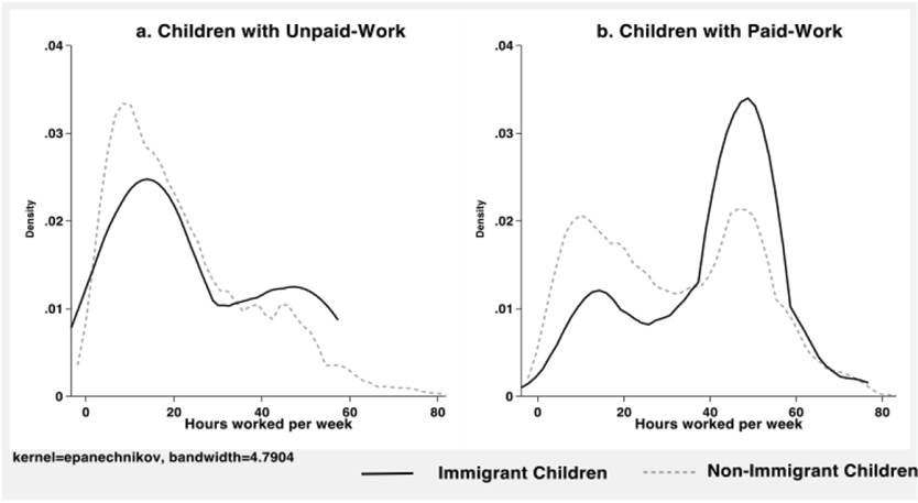
Source: Authors' calculation with data 2013 MTI-ENOE.
Figure 1 Children’s hours worked per week by paid/unpaid work and children’s migration status
The left panel of Figure 2 shows the percentage of child labour rates and school attendance by children's migration status. Most households, or 98.77%, are nonimmigrant households. The nonchild labour percentage differs between nonimmigrant and immigrant children by 3.4 percent (91.4% compared to 88.0%). The results show a larger percentage of child labour in newly arrived children than in nonimmigrant children (12.0% vs. 8.6%). Overall, the working rate among children is 8.6%, independent of household migration status.
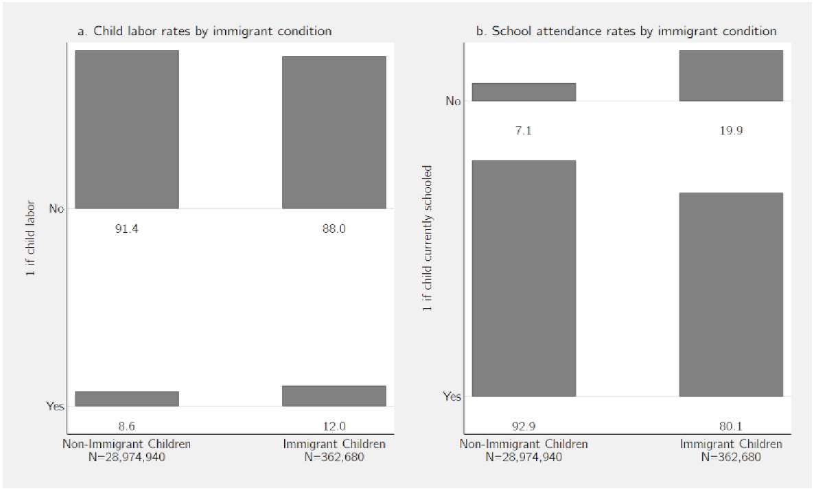
Note: Population weights used to compute the child population.
Source: Authors' calculation with data from 2013 MTI-ENOE.
Figure 2 Child labour rates and school attendance by child migration status
Figure 2 on the right side compares the schooling attendance by children's migration status. It seems that education could be one of the reasons for children to move to another place, as it was one of the main reasons to move. This result confirms that in Mexico, a larger percentage of immigrant children (19.9%) do not attend school than nonimmigrant children (7.1%). For all children, a lower percentage of recent immigrants attend school than nonimmigrants, which could be linked to less continuity in their educational trajectories due to more geographical movements and school changes. This evidence suggests that the self-selection of migrants could be related to their school attendance.
4. Methodology
The question examined is whether immigrant children living in newly arrived households are more likely to work than nonimmigrant children. The empirical strategy accounts for the endogeneity effect of migration and other unobservable factors affecting two decisions: the decision to engage in child labour and migrate. This paper models these two decisions as independent; however, unobserved factors affect child labour and migration decisions. These factors include the father's, mother's, and children's abilities, attitudes towards improving opportunities, and preferences for better quality schools.
The endogeneity of the migration process complicates the identification of the causal effect of migration on child development. Newly arrived households and members' self-select into this status based on observed and unobserved characteristics. The empirical strategy used is to separately estimate child labour and household migration determinants while considering that unobserved factors affect both decisions. The estimated model comprises two binary dependent variables for the outcome and selection equations. The recursive bivariate probit model uses two probit equations whose error accounts for the potential nonzero correlation of the error term in the two equations (Filippini et al., 2018). Estimating both equations as a system will not affect the consistency of individual probit estimates. See Greene (1998) and Maddala and Lee (1976) for more details about the recursive bivariate probit model.
The outcome equation has, as its dependent variable, Y1, representing the child labour variable, which takes a value of 1 and 0 otherwise, and the selection equation also has a binary dependent variable, Y2; an individual who is an immigrant child (new resident children are those children living in a new resident or migrant household) takes a value of 1 and 0 otherwise. Hence, the latent variable Y*i1 represents the decision about child labour, and the latent variable Y*i2 represents the decision to household migration. The setup for the model is as follows:
The model accounts for the effect of migration on child labour because Yi2 is also included in the first equation as an endogenous variable. This specification is a recursive bivariate probit model, where Xi1 and Xi2 represent row vectors of exogenous variables that determine the decisions to participate in child labour and to migrate, respectively. Then, β'1 and β'2 are the vectors of coefficients associated with explanatory covariates. Additionally, εi1 and εi2 are the random parts assumed to be jointly normally distributed with zero means, unit variance, and correlation (ρ). The recursive bivariate probit allows for accounting for the potential nonzero correlation (ρ≠0) of the error term in the two equations. If ρ≠0, then the treatment is endogenous, and joint estimation is required (Filippini et al., 2018). The procedure needs at least one different independent variable in the selection equation for identification purposes.
Another essential variable is the effect of children's school attendance on immigrant households' decisions. In equation (2), school attendance affects the decision to migrate. For example, a household can send their children away or migrate together to access school or a better school (Hashim, 2005). Additionally, parents who care more strongly about education may migrate to earn income to pay for schooling expenses (McKenzie and Rapoport, 2011). Following Bhalotra and Tzannatos (2003), school attendance is not in the outcome equation. Even though this does not entirely identify the causal effect, it affects both decisions to work and migrate.
The household composition has some implications. The absence of a male role model might have a detrimental effect on boys, causing them to reduce their school efforts because they anticipate migrating for low-skilled work in the future (Powers, 2011). Child labour and migration decisions are both made in the child's current household. Hence, the sample is divided into two groups: a) children living in a nuclear household (whether one or both parents are present) and b) children living in extended families (nonnuclear households). The dependent variables are the decision to send a child to work and the household migration decision, and the independent variables are the child's age and gender, the household size, the household composition, the household head's completed grades in school, the locality size, and the region.
5 Results
Table 3 shows the marginal effect, applying a simple probit model, while Table 4 shows the conditional marginal effect between child labour and household migration, accounting for the endogeneity effect. The results provide evidence that household structure is essential in the decision to migrate and in work. The results provide evidence of a direct relationship between child labour and household migration. The direction of the coefficient sign does not change whether we do not control for endogeneity in the Table 3 models (1)-(4) or control Table 4 models (5)-(8). Comparing the whole sample, the probability that a child works is estimated at 1.05 % if the individual is a new resident child. The coefficient becomes larger, 5.16%, when we control for endogeneity.
Table 3 Probit model analysis of the decision to participate in child labour (marginal effects)
| Model 1 Full sample |
Model 2 Hh with both parents |
Model 3 Hh with absent father |
Model 4 Hh with absent mother |
|||||
|---|---|---|---|---|---|---|---|---|
| Coeff. | S.E. | Coeff. | S.E. | Coeff. | S.E. | Coeff. | S.E. | |
| Child characteristics | ||||||||
| 1 if immigrant child | 0.0105** | (2.157) | 0.0242** | (2.525) | 0.0250** | (2.612) | 0.0242** | (2.522) |
| 1 if male child | 0.0359** | (28.514) | 0.0339** | (22.659) | 0.0340*** | (22.681) | 0.0339*** | (22.630) |
| Age | 0.0096*** | (6.870 | 0.0091*** | (5.403) | 0.0091*** | (5.405) | 0.0093*** | (5.482) |
| Age squared | 0.0002*** | (4.262) | 0.0002*** | (3.530) | 0.0002*** | (3.536) | 0.0002*** | (3.490) |
| Household characteristics | ||||||||
| 1 if nuclear household | -0.00114 | (-0.765) | ||||||
| 1 if Hh with both parents | -0.0122*** | (-5.761) | ||||||
| 1 if Hh with absent father | 0.0118*** | (5.445) | ||||||
| 1 if Hh with absent mother | 0.00812 | (1.362) | ||||||
| Household size | 0.00102** | (2.898) | 0.0037*** | (6.672) | 0.0036*** | (6.457) | 0.0027*** | (5.121) |
| Household dead characteristics | ||||||||
| 1 if Hh head employed | 0.0315*** | (16.883) | 0.0270*** | (10.394) | 0.0270*** | (19.372) | 0.0247*** | (9.612) |
| 1 if Hh has no schooling | Ref. | Ref. | Ref. | Ref. | ||||
| 1 if Hh head has partial primary school | -0.0146*** | (-5.632) | -0.0104** | (-2.838) | -0.0105** | (-2.861) | -0.0110** | (-3.003) |
| 1 If Hh head has full primary school | -0.0222*** | (-8.770) | -0.0218*** | (-6.151) | -0.0219*** | (-6.193) | -0.0226*** | (-6.384) |
| 1 if Hh head has partial secondary school | -0.0246*** | (-6.390) | -0.0240*** | (-4.961) | -0.0241*** | (-4.997) | -0.0251*** | (.5.192) |
| 1 if Hh head has full secondary school | -0.0346*** | (-13.648) | -0.0348*** | (-9.946) | -0.0350*** | (-10.006) | -0.0357*** | (-10.194) |
| 1 If Hd head has preparatory or more school | -0.0578*** | (-21.299) | -0.0571*** | (-15.630) | -0.0573*** | (-15.687) | -0.0587*** | (-16.080) |
| Locality size | ||||||||
| 1 if less than 2 500 inhab | Ref. | Ref. | Ref. | Ref. | ||||
| 1 if city with 100 000 or more inhab | -0.0237*** | (-14.609) | 0.0246*** | (-12.558) | -0.0247*** | (-12.565) | -0.0245*** | (-12.470) |
| 1 if city with 15 000 to 99 999 inhab | -0.0152*** | (-7.287) | -0.0170*** | (-6.750) | -0.0170*** | (-6.749) | -0.0169*** | (-6.703) |
| 1 if city with 2 500 to 14 999 inhab | -0.0156*** | (-7.659) | -0.0145*** | (-5.983) | -0.0145*** | (-5.987) | -0.0146*** | (-6.025) |
| Regions | ||||||||
| 1 if North | Ref. | Ref. | Ref. | Ref. | ||||
| 1 if Centre-North | 0.0149*** | (7.241) | 0.0132*** | (5.372) | 0.0132*** | (5.366) | 0.0134*** | (5.469) |
| 1 if Centre | 0.0150*** | (6.360) | 0.0157*** | (5.599) | 0.0157*** | (5.588) | 0.0163*** | (5.780) |
| 1 if Capital | -0.00112 | (-0.370) | -0.00127 | (-0.344) | -0.00131 | (-0.354) | -0.00118 | (-0.319) |
| 1 if Gulf | 0.0136*** | (6.035) | 0.0132*** | (4.877) | 0.0132*** | (4.882) | 0.0132*** | (4.849) |
| 1 if South | 0.0190*** | (8.462) | 0.0163*** | (6.038) | 0.0163*** | (6.042) | 0.0168*** | (6.184) |
| 1 if Pacific | 0.0318*** | (14.256) | 0.0308*** | (11.808) | 0.0308*** | (11.804) | 0.0312*** | (11.907) |
| Observations | 95,496 | 67,305 | 67,305 | 67,305 | ||||
| Log likelihood | -21,708.1 | -15,162.2 | -15,164.0 | -15,177.7 | ||||
| McFadden’s R2 | 0.202 | 0.194 | 0.194 | 0.193 | ||||
| R Count | 91.85% | 92.06% | 92.06% | 92.06% | ||||
Note: Marginal effects; t statistics in parentheses * p <0.05, ** p <0.01, *** <0.001
Source: Authors’ calculation with data from 2013 MTI-ENOE.
Table 4 Recursive bivariate probit model analysis of the decision to participate in child labour (marginal effects)
| Model 5 Full sample |
Model 6 Hh with both parents |
Model 7 Hh with absent father |
Model 8 Hh with absent mother |
|||||
|---|---|---|---|---|---|---|---|---|
| Coeff. | S.E. | Coeff. | S.E. | Coeff. | S.E. | Coeff. | S.E. | |
| Child characteristics | ||||||||
| 1 if immigrant child | 0.0516*** | (7.046) | 0.0748*** | (4.722) | 0.0988*** | (5.052) | 0.0928*** | (4.386) |
| 1 if male child | 0.0521*** | (9.904) | 0.0582*** | (6.211) | 0.0717*** | (6.630) | 0.0681*** | (5.806) |
| Age | 0.0144*** | (5.161) | 0.0159*** | (3.811) | 0.0196*** | (3.934) | 0.0190*** | (3.754) |
| Age squared | 0.00035*** | (4.214) | 0.00043*** | (3.324) | 0.00053*** | (3.366) | 0.00050** | (3.212) |
| Household characteristics | ||||||||
| 1 if nuclear household | -0.00173 | (-0.795) | ||||||
| 1 if Hh with both parents | -0.0231*** | (-4.229) | ||||||
| 1 if Hh with absent father | 0.0229*** | (4.060) | ||||||
| 1 if Hh with absent mother | 0.0152 | (1.260) | ||||||
| Household size | 0.0014** | (2.752) | 0.0064*** | (4.648) | 0.0076*** | (4.554) | 0.0055*** | (3.756) |
| Household dead characteristics | ||||||||
| 1 if Hh head employed | 0.0357*** | (8.733) | 0.0383*** | (5.399) | 0.0481*** | (5.636) | 0.0423*** | (5.002) |
| 1 if Hh has no schooling | Ref. | Ref. | Ref. | Ref. | ||||
| 1 if Hh head has partial primary school | -0.0184*** | (-5.345) | -0.0165** | (-2.743) | -0.0207** | (-2.791) | -0.0206** | (-2.825) |
| 1 If Hh head has full primary school | -0.0273*** | (-7.068) | -0.0329*** | (-4.591) | -0.0413*** | (-4.808) | -0.0403*** | (-4.474) |
| 1 if Hh head has partial secondary school | -0.0273*** | (-6.290) | -0.0337*** | (-4.282) | -0.0427*** | (-4.450) | -0.0418*** | (-4.197) |
| 1 if Hh head has full secondary school | -0.0431*** | (-8.364) | -0.0541*** | (-5.413) | -0.0676*** | (-5.755) | -0.0654*** | (-5.164) |
| 1 If Hd head has preparatory or more school | -0.0660*** | (-9.193) | -0.0851*** | (-5.875) | -0.106*** | (-6.320) | -0.103*** | (-5.524) |
| Locality size | ||||||||
| 1 if less than 2 500 inhab | Ref. | Ref. | Ref. | Ref. | ||||
| 1 if city with 100 000 or more inhab | -0.0350*** | (-8.536) | -0.0431*** | (-5.736) | -0.0530*** | (-6.053) | -0.0502*** | (-5.408) |
| 1 if city with 15 000 to 99 999 inhab | -0.0193*** | (-6.377) | -0.0262*** | (-4.739) | -0.0326*** | (-4.925) | -0.0308*** | (-4.502) |
| 1 if city with 2 500 to 14 999 inhab | -0.0197*** | (-6.583) | -0.0226*** | (-4.507) | -0.0282*** | (-4.670) | -0.0270*** | (-4.329) |
| Regions | ||||||||
| 1 if North | Ref. | Ref. | Ref. | Ref. | ||||
| 1 if Centre-North | 0.0236*** | (5.591) | 0.0241*** | (3.985) | 0.0295*** | (4.109) | 0.0288*** | (3.926) |
| 1 if Centre | 0.0244*** | (5.010) | 0.0299*** | (4.039) | 0.0364*** | (4.177) | 0.0361*** | (4.016) |
| 1 if Capital | -0.00112 | (-0.262) | -0.00202 | (-0.323) | -0.00257 | (-0.334) | -0.00219 | (-0.298) |
| 1 if Gulf | 0.0219*** | (4.872) | 0.0246*** | (3.728) | 0.0301*** | (3.831) | 0.0285*** | (3.645) |
| 1 if South | 0.0319*** | (6.136) | 0.0310*** | (4.259) | 0.0379*** | (4.415) | 0.0371*** | (4.204) |
| 1 if Pacific | 0.0586*** | (8.232) | 0.0637*** | (5.731) | 0.0769*** | (6.029) | 0.0743*** | (5.496) |
| Selection equation: New-resident child | ||||||||
| 1 if currently schooled*partial primary | -0.0149*** | (-5.347) | -0.0123*** | (-1.954) | -0.0152*** | (-1.910) | -0.0143*** | (-1.879) |
| 1 if currently schooled*full primary | -0.0166*** | (-4.920) | -0.0130*** | (-1.869) | -0.0162*** | (-1.826) | -0.0152*** | (-1.799) |
| 1 if currently schooled*partial secondary | -0.0159*** | (-5.186) | -0.0077*** | (-1.511) | -0.0096*** | (-1.486) | -0.0089*** | (-1.468) |
| 1 if currently schooled*full secondary | -0.0148*** | (-4.255) | -0.0132*** | (-1.735) | -0.0165*** | (-1.695) | -0.0154*** | (-1.673) |
| 1 if currently schooled*preparatory | -0.0144*** | (-4.029) | -0.0072*** | (-1.196) | -0.0089*** | (-1.181) | -0.0084*** | (-1.170) |
| Observations | 95,496 | 67,305 | 67,305 | 67,305 | ||||
| Log likelihood | -28,273.0 | -16,972.0 | -16,973.8 | -16.987.6 | ||||
| Rho (p) | -0.598 | -0.403 | -0.404 | -0.398 | ||||
| Chi2 | 47.79 | 53.23 | 53.51 | 52.16 | ||||
Note: Bivaritate probit model corresponds to conditional probability “Prob” [y1=1,y2=1|x1,x2]
Marginal effects; t statistics in parentheses * p < 0.05, ** p < 0.01, *** p < 0.001.
Source: Authors calculation with data from 2013 MTI-ENOE.
The simple probit model estimates could be biased downwards because they do not consider the effect of unobserved heterogeneity associated with migration decisions. The decision to migrate can be, in turn, correlated to the probability that children work. If we do not account for unobservable factors such as the ability of the parents or the child, then we ignore valuable information regarding education or the desire to improve life quality, but those are unobservable in our data. A way to account for this important information is by estimating a recursive system to identify joint decisions. We can have positive or negative selectivity depending on the quality or ability of the immigrants relative to the departure states. We can infer positive selectivity when accounting for the unobservable as the coefficients increase in magnitude in the controlled models. These results are consistent with those of Aguayo-Téllez and Martínez-Navarro (2013), who found evidence of selectivity in the case of internal migration in Mexico.
The coefficient of a nuclear household relative to an extended household is negative, indicating that it is a factor that may reduce child labour. However, it is not statistically significant when considering the whole sample. The nuclear household sample incorporates three possibilities: the results show that the probability that a child works - in an immigrant household - is positive and more prominent in magnitude. If both parents are present in the nuclear household, as in model (2), the probability of child labour and a new resident household is 2.42%. When controlling for endogeneity, it is even larger, 7.48%; see model (6). Comparing uncontrolled models where the father is absent, as in model (3), with the mother's absence, model (4), the probability that an immigrant child works is larger when the father is absent.
The results show a similar pattern in the models that account for endogeneity, models (7) and (8). However, the coefficients are considerably larger than in other models, 9.88% and 9.28%. Without conditioning to new resident children, the probability of child labour is lower if the household is nuclear-with both parents living in the household-but larger if the father is absent; these coefficients are smaller in magnitude than in the case of new resident children. These results provide evidence that it is more likely that children will work if they are new in the neighbourhood and live in households with the mother acting as the head of the household. The joint probability between child labour and migration accounts for the unobservable factors affecting both decisions and delivers better-estimated coefficients. It follows that the correlation (ρ) coefficient is statistically significantly different from zero and that the log-likelihood tests are larger than the probit models, which do not control for endogeneity.
In general, the control variables' coefficients for comparable models have the same direction for the probability of child labour. In the biprobit models, the coefficients are larger in magnitude and have smaller standard errors relative to the probit models. For this reason, the interpretation is based on models (5) to (8) in Table 4. The coefficients shown in model (5), which considers the whole sample, are smaller than the estimated coefficients obtained for nuclear households. When comparing the coefficients for nuclear households, the largest coefficients, in terms of the absolute value, are estimated for nuclear households with the father absent.
In contrast, the lowest coefficients are for nuclear households with the mother absent. This result is related to previous studies that suggest that the probability of child labour for a new resident child is higher than that of a habitual resident child (Grootaert and Kanbur, 1995; Jensen and Nielsen, 1997; Rosati and Rossi, 2003). A binary variable identifies whether the household's head is working. In model (6), both parents are present, and they self-declare which one is the head of the household. In the father's absence, the mother is the head of the household, model (7); in contrast, the father is the head of the household if the mother is absent, model (8). The results imply that if the head of the household is employed, the probability of child labour increases, although this effect seems counterintuitive. This is consistent with the argument of Basu and Van (1998) that child labour and adult work are complementary, particularly for migrant households.
The probability of child labour decreases if the head of household’s education level increases relative to the head of household with no education. Consistent with Hanson and Woodruff (2003) and McKenzie and Rapoport (2011), the probability of child labour decreases by a larger magnitude in localities with more than 100 000 inhabitants relative to localities with less than 2 500 inhabitants. Thus, the probability of child labour is larger in rural localities than in urban localities. The Pacific and South regions have the largest child labour probabilities relative to northern states. Overall, it is remarkable that the probability of child labour is approximately 7.69% in households with the father's absence in the Pacific region relative to the northern states. The probability of child labour is larger in the Centre and North-Centre than in the northern states. Only in the capital, Mexico City, and the State of Mexico is the probability of child labour lower than in the Northern states, although none of the coefficients was statistically significant.
Finally, the biprobit models (Table 4) account for the indirect effect of education on child labour. The interaction set of binary variables combines current school attendance and the highest level of education. As expected, there is an inverse relationship between both variables. However, this effect is not homogeneous for specific educational outcomes. Older children may be more likely to engage in work than attend school.
Figure 4 shows that the predicted child labour and children's immigration status probabilities differed across regions. We also showed confidence intervals of 95 percent at the mean values of other covariates. In general, the Capital Region has the lowest probability of child labour. The regions with the highest child labour rates are the Centre-North, North, and Pacific regions. However, the child labour probabilities by migration status are only statistically significant in the North, North-Centre, and South regions. Migrant children in the North region have statistically significative highest child labour rates compared to nonimmigrant children. This result is related to previous evidence indicating migratory flows of families to border states in search of job opportunities (Aguayo-Téllez and Martínez-Navarro 2013).
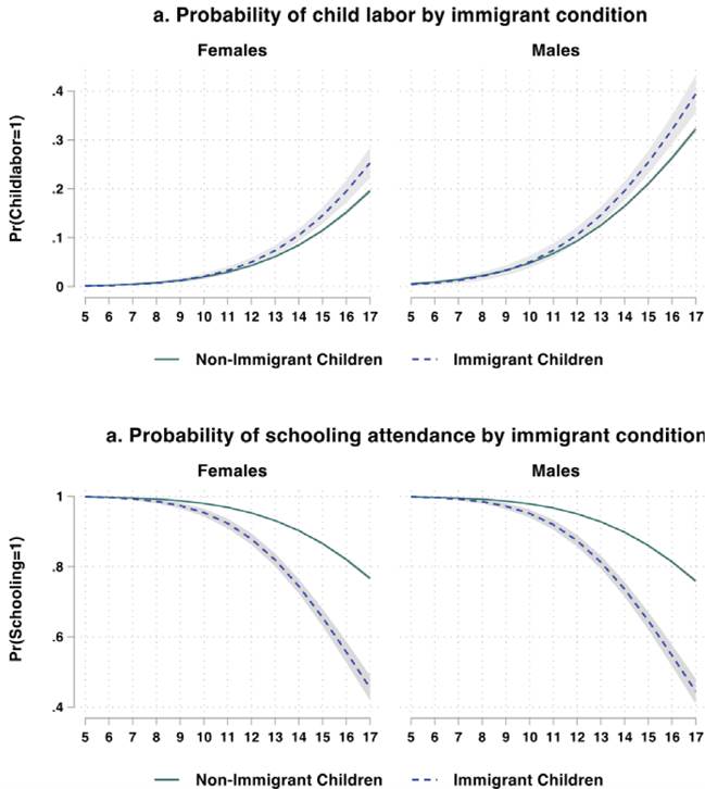
Notes: Predicted probabilities and 95 percent confidence intervals were calculated at mean values of other covariates. Probabilities are based on coefficients reported in Model 5 of Table 4. The y-axis indicates the children's age.
Figure 3 Gender differences in the predicted probabilities of child labour and schooling attendance by immigrant condition
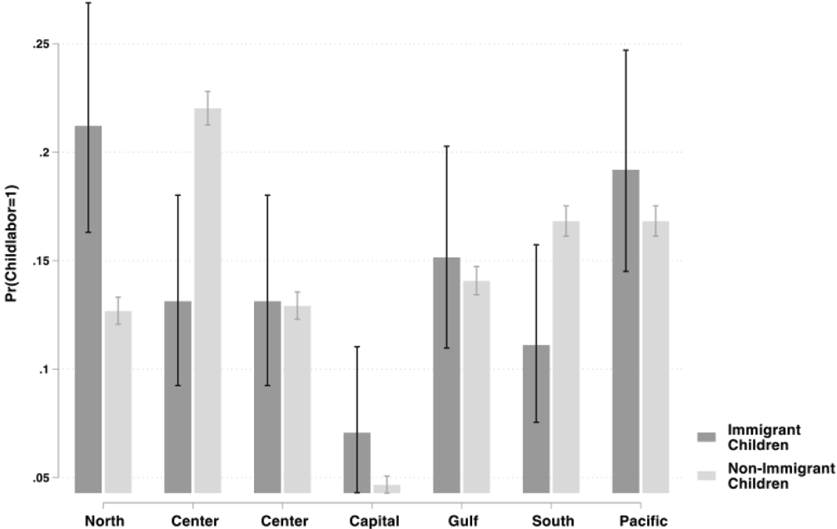
Notes: Predicted probabilities and 95 percent confidence intervals were calculated at mean values of other covariates. Probabilities are based on coefficients reported in model 5 of Table 4. The x-axis indicates the region of current residence.
Source: Authors' calculation with data from 2013 MTI-ENOE.
Figure 4 Predicted probabilities of child labour by region
The predicted probabilities according to immigration status show that in the North and Pacific regions, immigrant children are more likely to work than nonimmigrants. Factors related to the new environment, such as regional differences in the level of economic development that demand work and attract migrants from other states and higher costs of living in destination regions, may pressure immigrant families to send their children to work. The result is high opportunity costs of keeping children in school among the new-resident households. Unfortunately, from the MTI-ENOE, we do not know the origin of immigrant households to infer how these differences affect them directly.
Figure 3 shows gender differences in predicted probabilities of child labour and schooling attendance by children’s migrant status. The probabilities of child labour and school attendance increase and decrease as long as children's age increases. According to the results, the broader gaps are in the likelihood of attending school, with migrant children being less likely to continue their education. Although the gap is smaller between the two groups, migrant children are more likely to engage in child labour. We find statistically significant differences for children older than 15 years old. Based on these differences, the results suggest a disadvantage for immigrant children compared to nonimmigrant children. This situation corresponds to the migration status itself and the simultaneous combination of factors that impact child labour and schooling that presumably most affect immigrant children.
6. Conclusion
One of the main reasons for household migration is the search for better welfare opportunities for household members. The decision to migrate is an individual and family decision, and displacement may depend on conditions and factors analysed from a cost-benefit perspective, in which income and expected well-being are the main determinants. In the case of internal migration, this corresponds to changes in the residence of households within the same country. Households move in search of social and economic benefits and better wages because of the unequal distribution of income between regions or states in Mexico.
In this paper, we study the relationship between domestic household migration and child labour in Mexico. We control endogeneity by accounting for unobservable factors affecting child labour and migration using a recursive bivariate probit regression. The substantive findings are that, compared to nonmigrant children, immigrant children have a greater probability of being involved in child labour. This condition is robust to various specifications and controls. In addition, when comparing the employment conditions of children working in the country, we find that immigrant children are more likely to work long hours and receive lower wages than nonmigrant children.
For nuclear households, this probability increases when the father is absent in households where the mother is the head of the household. Households with the mother as the head have lower incomes than households where the father is the head of the household. These results are consistent with previous evidence on child labour, namely, that the probability of working increases with age, is higher for boys, and is higher in rural areas. New resident children are a vulnerable group: even if they seem to have a higher level of education than nonmigrant children, they work longer hours for payment, at least 35 hours per week. Another significant result is the existence of a trade-off between school attendance and child labour, as suggested in the literature review.
Children's early involvement in child labour is a complex problem that affects children's current well-being and expected future well-being, and the analysis of its determinants in the context of household domestic migration can guide the knowledge and impact of these population movements, as well as the attention to specific needs in the places of origin and destination. Overall, if the reduction of child labour is a policy goal, removing barriers to schooling attendance is one of the main areas to eradicate child labour. This educational policy for migrant children should focus on supporting maintenance in school and cover differences in the academic background given the differences in educational quality in Mexico.
There is a need to implement programmes that focus on attracting children to school by reducing administrative difficulties in enrolling and retaining immigrant children by filling new students' learning gaps. Teachers and schools are the links to understanding children's issues at the new location. First, parents should be supported in the documentation and registration process; flexibility is required when the school year has already started. Second, children should be given remedial programmes to standardize and normalize their level of knowledge. Third, teachers should be trained to adapt their teaching material based on the educational lags of these children.
As in other developing countries, in Mexico, child labour still occurs. Among children, immigrant children are the most vulnerable. Child labour might be an obstacle to social and economic development and drive poverty's intergenerational transmission. Child labour is a complex issue with longer-run implications for school-aged children and child well-being. According to the International Labour Organization (ILO), child labour violates human rights irrespective of migration status or age. Therefore, the Mexican government should ensure the implementation of the United Nations Conventions on the Rights of the Child and the ILO Child Labour Conventions (No. 138 and No. 182). Additionally, the government should develop labour monitoring mechanisms and oversee child labour in the informal economy, where most children work. Additionally, there should be a particular programme for those arriving in new households to facilitate the assimilation process.