


 nueva página del texto (beta)
 Inglés (pdf)
 Artículo en XML
 Referencias del artículo
 Enviar artículo por email
 Citado por SciELO
  Similares en
SciELO
Similares en
SciELO 
 Permalink
1. Introduction
The unemployment rate is high in the majority of European Union member states. To reduce unemployment, flexibility of labor has been proposed by orthodox scholars as a solution. In this article, we show that unemployment is not determined by variables such as real wage and social protection but rather by macroeconomic variables such as capacity utilization, inequality, and whether or not the countries are core or peripheral1 from to 2010 to 2012.
The article is organized as follows: in section 2, we describe the unemployment rates in Europe for the last 40 years; in section 3, we analyze whether or not unemployment is determined by high real wage as the neoclassical theory predicts; in section 4, we show a Bayesian method for selecting variables; and in section 5, we relate unemployment rate, capacity utilization, inequality, and core/peripheral countries using appropriate econometric techniques, section 6 is dedicated to concluding remarks.
2. Unemployment rate trends
Since the beginnings of the 1970s, the unemployment rate has been increasing in countries in the European Union (Duménil and Lévy, 2007; Armstrong, Glyn and Harrison, 1991; Glyn, 2006; Atkinson, 2015). Figure 1 shows the unemployment for three countries, Germany, France, and the UK (UK1), based on data from the International Labor Organization (ILO).2 Observing figure 1, we arrive at the following conclusions: at the beginning of the 1970s, the unemployment rate in Germany was less than 1 percent, whereas in the United Kingdom it was nearly 4 percent. However, the unemployment rate skyrocketed during the 1980s and the 1990s in Germany and France. According to Glyn (2006), the unemployment rate increased fivefold from the 1960s to the 1990s throughout Europe. Setting aside Germany, none of the other countries have achieved consistent reductions in the unemployment rate since the end of the 1990s. It is clear that the current unemployment rates are higher than the rates that prevailed at the beginning of the 1970s.
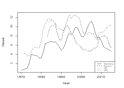
Source: ILO (2017) for Germany and France and UK1 and Office for National Statistics (2016) for the UK2.
Figure 1. Unemployment rate in Germany, the United Kingdom, and France
In addition, there has been a loss of manufacturing jobs, disempowerment of the unions, and a decline in the average hours of work (Glyn 2006; Eichhorst, Max and Wehner, 2016). Concomitant to this trend, instead of permanent jobs, the percentage of temporary jobs has increased sharply during the last 10 years among the young labor force (age 15-24) in countries such as Croatia, Cyprus, the Czech Republic, France, Germany, Hungary, Ireland, Italy, Luxemburg, Malta, the Netherlands, Poland, Portugal, and Slovenia (Eichhorst, Max and Wehner, 2016; Eichhorst and Marx 2011). Finally, according to the Organization for Economic Cooperation and Development, OECD (2015), the average probability of moving from unemployment to having a permanent job is only 50 percent in most European countries, and in countries such as Italy and Spain is approximately 40 percent and 25 percent, respectively.
3. The relationship between real wage and the unemployment rate
In the orthodox argument, the supply of labor and the demand of companies for labor determine real wage (the market labor). If unemployment exists, it is because the supply of labor is fixed and expensive. Unemployment occurs when real wage and social protection are higher than marginal productivity of labor (Hopenhayn and Rogerson, 1993; Caballero and Hammour, 1997). A greater flexibility with respect to the supply of labor is, therefore, proposed by orthodox scholars to encourage the level of employment (OECD, 1994; Krueger 2002; IMF, 2003; Gadatsch, Stahler, and Weigert, 2016). At the end of 1990s, and throughout the 2000s, to make the supply of labor more flexible, several labor reforms were established in Europe, for example, the Hartz Labor in Germany in 2002 and the Khomri Law in France in 2016, and zero-hour contracts that have been carried out in the UK since the 1990s (Cukier, 2016).
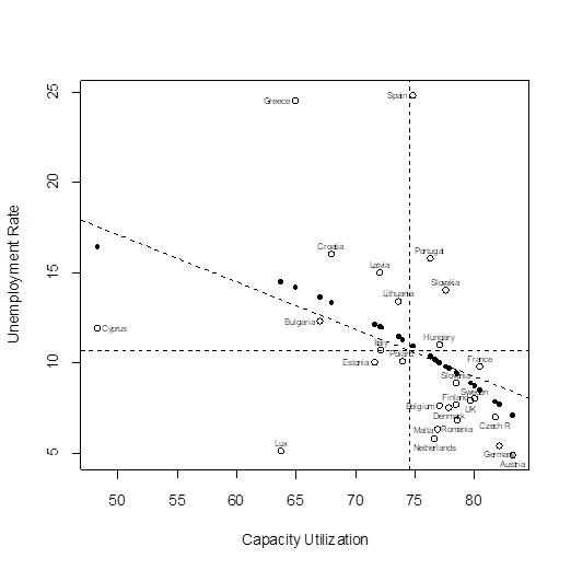
Theoretical as well as empirical evidence challenges the assertion that the labor market determines the real wage and the volume of employment. First of all, as Keen (2011) has shown, marginal productivity of labor equaling real wage is not economic rule. If national income equals profit rate multiplied by the stock of capital plus the wage rate multiplied by the volume of employment, then the marginal productivity of labor equals the real wage plus profit rate multiplied by the change in the stock of capital plus the stock of capital multiplied by the change in the profit rate, and plus the volume of employment multiplied by the change in the wage. For this reason, marginal productivity of labor is difficult to observe. Second, past evidence and that from recent years have led to a rejection of the orthodox assertion (Glyn, 2006). It is a stylized fact that during the golden years (after WWII to 1974), along with rising wages, increasing levels of employment and social protection occurred. Besides, there is currently no evidence that a high real wage is related to unemployment in the European Union (Froyen, 2013). Figure 2 plots the unemployment rate and real wage per hour in 2012 for the 28 countries of the European Union plus Turkey, Norway, and Iceland.3 Figure 2 also shows the mean of real wage per hour (vertical dotted line) and the mean of unemployment rate (horizontal dotted line). Five results can be observed:
The neoclassical hypothesis does not hold. High real wage is not related to a high unemployment rate; in contrast, concomitant to high wages, low unemployment rates seem to occur. A line with a negative slope is the best description of these observations.
Core countries of Europe such as France, Sweden, Finland, the United Kingdom, the Netherlands, Denmark, Belgium, and Germany have high real wage and a low unemployment rate; only Italy is borderline between high real wage and a low unemployment rate.
Ireland and Spain have high levels of unemployment and high real wage.
Nine countries (Greece, Croatia, Portugal, Latvia, Slovakia, Cyprus, Lithuania, Bulgaria, and Hungary) present low real wage and high unemployment level.
Only 7 countries have low real wage and low levels of unemployment (Poland, Estonia, Slovenia, Turkey, the Czech Republic, Malta, and Romania); all these countries are peripheral. Even though the relationship between unemployment rate and real wage is significant, R square is a low 17 percent. Removing the outliers such as Spain, Greece, and Romania produces an R-square of 31 percent. This evidence shows that the neoclassical hypothesis did not hold during 2012.
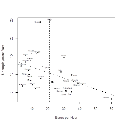
Source: Author´s elaboration with data from Eurostat, 2016.
Figure 2. Unemployment rate and real wage per hour, 2012
The evidence favors classical, Marxian, and post-Keynesian scholars who claim that low wage occurs concomitant to high levels of unemployment (Kaldor, 1940, Harrod, 1939; Harrod, 1958; Minsky, 2013; Shaikh, 2013). As is well known, Marx believed that the reserve army of labor exerts a downward pressure to wages. Conversely, increasing employment may occur with increasing real wage as long as technological change holds constant (Marx, 1946). Also, neither Keynes nor Kalecki thought that high real wage caused unemployment (see Harrod, 1958; Keynes, 1964; Kalecki, 1977).
Finally, rigidities in the labor market encompass not only real wage but also social protection. According to some economists, the state spends too much on healthcare and unemployment benefits (Caballero and Hammour,1997). Therefore, to reduce the cost of labor, social protection has to be limited. Figure 3 shows social protection as percent of GDP and the unemployment rate; no trend is evident. However, it is obvious that core countries have a lower unemployment rate along with higher social protection.
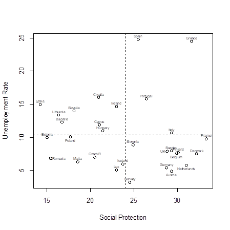
Source: Author´s elaboration with data from Eurostat, 2016.
Figure 3. Unemployment rate and social protection (% of GDP), 2012
Thus, instead of looking for variables such as real wage and social protection in determining the unemployment rate, we must turn to macroeconomic variables such as inflation, capacity utilization, and inequality. The first variable is highlighted by the orthodox approach, whereas the latter variables are the focus of a heterodox approach. We proceed to review the three variables, arguing that capacity utilization and inequality play a big role in explaining unemployment.
4. A statistical method for selecting variables
Instead of variables such as real wage and social protection determining the unemployment rate, we favor macroeconomic variables such as capacity utilization and inequality (Foley and Michl, 1999; Galbraith, 1997; Chick, 2000; Minsky, 2013; Shaikh, 2016). To strengthen our theoretical insights, we use a Bayesian method to select variables. Under this methodology, which follows Bayes’ theorem, we distinguish the correct models and the variables that integrate these models given the data. Then, following Raftery, Painter and Volinsky (2005) (see also Albert, 2007), we have:
P(Modelk/Data) holds for the posterior probability of a modelk being correct given the data. Meanwhile, on the right side of the equation, the numerator consists of the prior probability of a k model (P(Model)) multiplied by the likelihood function of each model P(Data/Modelk), and the denominator consists of the total sum of all the k possible models in the numerator. We obtain the results listed in table 1 by applying this technique to money wage, real wage, education (tertiary education as percent of educated individuals age 15 to 64), inflation rate, social protection (as a percent of GDP) (SP), GNP (Gross National Product) per capita (GNP), capacity utilization (current level of capacity utilization in the manufacturing industry) (CU), inequality (Gini coefficient of equalized disposable income before social transfer), and a dummy variable, which is code 1, if the country is peripheral, and 0 if the country is core (Pérez-Caldentey and Vernengo, 2012) . Then, the best models are:
Table 1. Summary of statistics, data for 2012
| Variables | P | Mean | Model1 | Model2 | Model3 | Model4 | Model5 |
|---|---|---|---|---|---|---|---|
| Intercept | 100.0 | -19.0 | -17.71 | -30.27 | -22.12 | -32.83 | -12.46 |
| Money wage | 26.8 | 0.78 | 12.49 | ||||
| Dummy var | 93.0 | 11.0 | 11.04 | 11.87 | 11.72 | 0.39 | 11.00 |
| Inequality | 73.1 | 0.32 | 0.41 | 0.40 | 0.34 | 0.12 | 0.36 |
| Education | 16.1 | 0.016 | |||||
| Inflation | 25.7 | -0.28 | -1.05 | -0.83 | |||
| Real wage | 25.9 | -.0.72 | 0.43 | ||||
| SP | 87.0 | 0.48 | 0.59 | 0.51 | 0.59 | ||
| GNP | 13.2 | -0.00 | -0.17 | ||||
| CU | 38.2 | -0.059 | 4 | -0.15 | |||
| nVariables | 0.658 | 3 | 4 | 4 | 5 | ||
| R2 | -14.86 | 0.607 | 0.632 | 0.631 | 0.673 | ||
| BIC | -14.51 | -12.99 | -12.87 | -12.8 |
Source: Author´s elaboration with data from Eurostat, 2016, R 3.3.0.
P holds for the posterior probability that a given variable appears in a model, mean is the average of the variable’s value in all the models, and Model1 to Model5 are the best models fitted according to R-square and to the Bayesian Information Criterion (BIC). The first model with the dummy variables core/periphery, inequality, social protection, and capacity utilization is the most appropriate. In this first model, R-square is 0.658, and the BIC is -14.86.
A very polemic variable such as inflation appears in model number 5. Therefore, low levels of inflation are not associated to high levels of unemployment, and high levels of inflation are not related to low levels of unemployment for the year of 2012. This fact contradicts the existence of a tradeoff between unemployment and inflation in the short run, and the existence of a vertical Phillips curve in the long run (Friedman, 1968). Figure 4 shows no relationship can be established between the unemployment rate and the inflation rate. The only fact that can be supported is that core countries present low inflation and unemployment. However, this result must be interpreted cautiously because we are using only one year, and the Philips curve is supposed to hold in the long run. We do not analyze a more extensive period because of information availability.
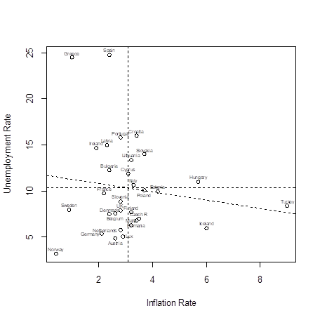
Source: Author´s elaboration with data from Eurostat, 2016.
Figure 4. Unemployment rate and inflation rate, 2012
5. The relationship among capacity utilization, inequality, and the unemployment rate
After identifying the most important variables for determining the unemployment rate, we run a linear regression with inequality, social protection, and the dummy variable peripheral/core country. We find that the inequality result is not significant; subsequently, we add a quadratic term in the variable capacity utilization to regression (this is our first model). As can be seen in figure 5, in spite of the presence of outliers, regarding capacity utilization, a curve fits the observations more properly than a line.
Source: Author´s elaboration with data from Eurostat, 2016.
Figure 5. Unemployment rate and capacity utilization, 2012
Then, the equation for this first linear regression is as follows:
The results can be seen in table 2: R-square is 70 percent. The BIC for the first model is 155.88, and for the second model is 151.58. In addition, the null hypotheses are accepted for all diagnostic tests (see table 3).4 Examining the coefficients, we reach the following conclusions: 1) if capacity utilization increases, unemployment increases until reaching some point; beyond this point, if capacity utilization increases, unemployment declines; 2) peripheral countries are expected to have 10.5 higher levels of unemployment than core countries; and 3) a 1 percent increase in social protection as a percent of GDP increases the unemployment rate in 0.70 percent.
Table2. Regression results. First model
| Coefficient | Std. error | t value | Probability | |
|---|---|---|---|---|
| Intercept | -93.525391 | 33.375809 | -2.802 | 0.010384 |
| CU | 2.679636 | 0.978519 | 2.738 | 0.011995 |
| Cu | -0.021130 | 0.007242 | -2.918 | 0.007974 |
| Periphery | 10.459009 | 1.888612 | 5.538 | 0.000045 |
| SP | 0.695879 | 0.152108 | 4.575 | 0.000148 |
Source: Author´s elaboration with data from Eurostat, 2016, R 3.3.0.
Table 3. Diagnostic tests. First model
| Diagnostic test | Probability |
|---|---|
| Heteroscedasticity | 0.6453 |
| Normality | 0.5138 |
| Functional Form | 0.3737 |
| Autocorrelation | 0.1511 |
Source: Author´s elaboration with data from 2016, R 3.3.0.
To corroborate that our results do not hold only for the year of 2012, we add other years. Unfortunately, we have data only for information only for the 2010-2012 period. With this panel data, we run a second regression with the following equation:
The subscripts i and t hold for country and time, respectively. Instead of letting the intercept change, as was the case in the previous model (equation 2), we let the slope change in an interaction between social protection and the dummy variable core/periphery. This change is due to the level of the unemployment rate, which is different for core and periphery countries depending on the variable social protection. The argument of this approach is presented in figure 6. After plotting unemployment rate and social protection as a percent of GDP again, and identifying core and peripheral countries, we find the following: core countries spend more in social protection than peripheral countries, but within core countries, increasing social protection results in a higher unemployment rate. Meanwhile, peripheral countries spend less in social protection than the core countries, but within peripheral countries, increasing social protection also results in a higher unemployment rate (see the two regression lines in figure 6). This result is more significant for the panel data model than for the linear regression for the year of 2012. Another change in the second model is the omission of the quadratic term in the variable capacity utilization because it is not significant. Finally, not considering heteroscedasticity, the model fulfills all the diagnostic tests (see table 4). To deal with heteroscedasticity, we use a robust covariance matrix. The regression results are presented in table 5.
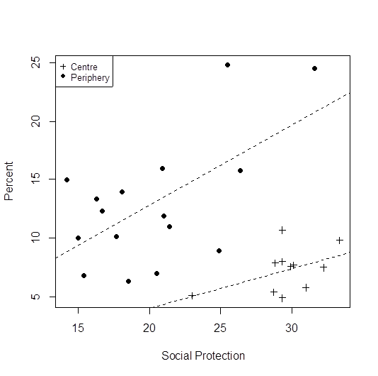
Figure 6. Unemployment rate, social protection (% of GDP), and the identification of core and peripheral countries
Table 4. Diagnostic tests. Panel regression, random effects. Second model
| Diagnostic test | P-value |
|---|---|
| Testing for random effects | 0.0000 |
| Cross-sectional dependence | 0.3726 |
| Serial correlation | 0.2501 |
| Heteroscedasticity | 0.01084 |
| Normality | 0.1198 |
Table 5. Regression results. Panel data, 2010-2012, random effects. Second model
| Variable | Coefficients | Std. Error | t value | P-value |
|---|---|---|---|---|
| Intercept | -16.121524 | 7.716832 | -2.0891 | 0.0400426 |
| CU | -0.18550 | 0.047301 | -3.9217 | 0.0001912 |
| Inequality | 0.594136 | 0.142336 | 4.1742 | 0.0000788 |
| SPcore | 0.293516 | 0.083141 | 3.5303 | 0.0007087 |
| SPPeriphery | 0.657548 | 0.132039 | 4.9799 | 0.0000038 |
As can be seen in table 5, the value of the intercept, the B1, and the B2 resemble the values presented in table 1. The slope of capacity utilization is negative. The increase in capacity utilization, therefore, is a reduction in unemployment, as is predicted by post-Keynesian scholars. Furthermore, the slope of inequality is positive, so an increase in inequality results in an increase in unemployment, as is predicted by some Marxian scholars. Therefore, in this statistical exercise, we find evidence supporting the two heterodox approaches. On the one hand, for post-Keynesians, capacity utilization can vary in the short run, and when capacity utilization declines, utilization of capital and labor also declines (see Foley and Michl, 1999; Minsky, 2013). On the other hand, for some Marxians, capacity utilization tends to be normal, and therefore inequality, expressed as a variation of the wage share, is negatively related to unemployment (Shaikh 2013, 2016).5
6. Conclusion
The objective of this article was to relate the rate of unemployment to capacity utilization, inequality, and whether or not the countries were core or peripheral in the short run. Our main findings were the following: 1) the unemployment rate is not related to real wage for the 2010-2012 period--if a relationship existed, it favored the classical argument and not the neoclassical; 2) the rate of inflation is not related to the rate of unemployment as demonstrated by a cross-sectional data for the 2010-2012 period, but we were not able to expand this analysis to additional years because of information availability; and 3) social protection is positively related to the rate of unemployment. This last finding does not support the orthodox argument that the welfare state must be dismantled. The reason for increases in social policies has been the neoliberal policies that have led to increased unemployment, and, therefore, social protection has been a defensive strategy to manage the pernicious effects of labor flexibility.
As Glyn (2006) has pointed out, market policies have not significantly increased the level of employment in any OECD country. In the short run, therefore, theoretical and statistical arguments favor the reduction of inequality and the rise of capacity utilization as the best approach to creating jobs. However, the disparities between core and peripheral countries also have to be addressed.

