


 nueva página del texto (beta)
 Inglés (pdf)
 Artículo en XML
 Referencias del artículo
 Enviar artículo por email
 Citado por SciELO
  Similares en
SciELO
Similares en
SciELO 
 Permalink
Introduction
In recent years, agricultural activities have caused an over-extraction and overuse of groundwater, which could eventually lead, in the short term, to an increase in the presence of toxic elements in crops and soil salinization, endangering the long-term availability of agricultural food products (Ebrahimia et al. 2016, Yu et al. 2021). It is estimated that the salinization of irrigated agricultural soils has caused the degradation of agricultural land, leading to production losses of 27.3 billion dollars a year (González-Acevedo et al. 2016). The quantity and quality of irrigation water is a crucial factor in agricultural production for both the short and long term (Loera-Alvarado et al. 2019, Chenchen et al. 2020, Mohammadi et al. 2021).
Evaluating the quality of agricultural water must into account its chemical characteristics, for example, the type and quantity of anions and cations present in it (Pacheco et al. 2004, Mohammadi et al. 2021). The chemical parameters of water quality can be incorporated and interpreted through the use of indexes and graphical methods (Güngör and Arslan 2016). Parameters and indexes such as CE, chlorides, sodium absorption ratio (SAR), potential salinity (PS) and effective salinity (ES) (Palacios and Aceves 1970) provide clear mathematical values that can be easily interpreted and help in decision-making processes related to the proper use of water (Delgado et al. 2010, Yu et al. 2021). Similarly, graphical representations of the chemical properties of water Piper diagrams (Piper 1944) and of the salinity and sodicity of irrigation water (Delgado et al. 2010. Bautista et al. 2015) can be used to define water types and the risk of salinity and sodicity, respectively.
Studying, analyzing and evaluating large datasets on water quality to build indexes and graphs demand considerable time as well as chemical and agronomic knowledge (Bautista et al. 2015, WH 2020). Furthermore, the management of data may be exposed to human errors. The process of analyzing irrigation water quality data can be automated through the use of software. The objective of this work was to describe the functions of the agriwater software in order that irrigated agriculture has a less negative impact on the environment and a better impact on agricultural production.
Materials and methods
Calculation and conversion of chemical units
The input variables consist of the following physico-chemical parameters: CE, Ca2+, Mg2+, Na+, K+, CO3 2−, HCO3 −, SO4 2−, Cl− NO3−, ∑ Cations, ∑ Anions.
The different calculations were done in the following order: conversion of units, classification of types of water, classification of salinity risks according to the diagram of salinity and sodicity, and trend analysis. The following equations were used to convert data units and to calculate the different water quality indexes (Delgado et al. 2010):
Unit conversion equations.
Conversion of mg L-1 into mmol L-1.
Conversion of mg L-1 into meq L-1.
Conversion of mg L−1 into meg L−1
Conversion of meq L−1 into mmol L−1.
Conversion of mmol L−1 into meq L−1.
The SAR index is calculated by the following equation:
The concentrations are expressed in meq L−1.
The potential salinity (PS) index is used to estimate the risk caused by a high
concentration of salts in solution (CI- and
The equation for calculating this index is:
The index of effective salinity (ES) provides a more accurate estimation of the risk cause by an increase in the osmotic pressure of the soil solution when high concentrations of carbonates and bicarbonates are present. These conditions cause calcium and magnesium carbonates to precipitate, and thus stop raising the osmotic pressure of the solution. This process is most noticeable when water has high concentrations of carbonates and bicarbonates. Water can be classified according to the ES into the same categories as the PS (Palacios and Aceves 1970). This index is calculated using the following conditions and equations:
Concentrations are expressed in meq L−1
The sodium adsorption ratio and electrical conductivity are parameters required to determine the quality of water in terms of their use for irrigating certain types of crops. The diagram of salinity and sodicity is used for this.
The diagram is divided into four levels according to the values of the sodium adsorption ratio expressed in (mmolc L−1)0:5 and the values of electrical conductivity expressed in dS m-1 at 25 °C, classifying the samples according to their values (low, medium, high and very high), which determine what type of water can be used with a certain crop.
Graphical methods
The diagram of salinity and sodicity represents the relationship between the sodium absorption ratio and electrical conductivity. The sodium absorption ratio divides the diagram into 4 regions: a) low: 0-10; b) medium: >10-18; c) high: >18-26; d) very high: >26-30. Likewise, electrical conductivity divides the diagram in 4 other regions: a) low: 0-0.250; b) medium: 0.250-0.750; c) high: 0.750-2.250; and d) very high: 2.250-5.0 dS m-1, defining a total of 16 types of irrigation water. With these parameters, the Agriwater software can make a plot, determining the number of pixels that correspond to each region and placing a dot when the parameters intersect, thus determining the type of water that corresponds to each of the n samples stored in the software, as well as the risk of salinization. The results of the classification are shown in tabular format and can be easily exported to an .xls file.
The Piper diagram determines the type of water, showing the major cations and anions contained in the sample, which is useful to determine the proper use of water. The diagram is formed by two triangles and a rhombus; the triangles represent the cations and anions, respectively, while the rhombus represents the type of water.
The operation of the software is based on the distribution of the proportions of ions contained in the sample, representing them in the diagram as percentages. Using these values, the software determines the proportion of pixels that correspond to each triangle, representing the intersection of all values with a dot. The points at which both triangles
intersect determine the values of the rhombus and the type of water.
Time series analysis
The Mann-Kendall test (MK test) was used for trend analysis (Mann 1945, Kendall 1975); this method has been widely described by (Castañeda and González 2008), as shown below.
The MK test begins by comparing the data from the most recent time series with previous values. A score of 1 is given if the most recent concentration value is higher than the previous one; if it is lower, the score is -1. The total score for the time series is the MK statistic, which is compared with a critical value to verify that the data show an upward or downward trend (Castañeda and González 2008). The analysis process is done as follows:
The n data pairs (x1, y1), (x2, y2), ...(xn, yn) are indexed according to the magnitude of the value of x, such that x1 ≤ x2 ≤...≤xn, with yi as the value of the dependent variable corresponding to x i .
All ordered n (n-1)/2 pairs of yi values are examined. Let P be the number of cases in which yi > yj (i>j), and let M be the number of cases in which yi < yj (i>j).
The statistics of the test is defined by S = P-M For n>10, the test is computed using the normal approximation. The standardized test statistic is calculated:
The null hypothesis is rejected at a level of significance of α if |Z|>Z(1-α)/2, where Z(1-α)/2 is the value of the standard normal distribution with a probability of exceedance of α/2. For example, at α= 0.05, the null hypothesis would be rejected for |Z|>1.96. In the case that some x and/or y values are tied, the formula for Var (S) is modified. If the sample size is less than 10, it is necessary to use tables for the statistic S.
The Kendall t correlation coefficient is defined as:
As with other types of correlation coefficients, π can only take values between -1 and 1; the sign indicates the sign of the slope of the relationship, and the absolute value indicates the strength of the relationship. Because the test only considers data rows, it can be used even in cases where some of the data are rejected. This is an important feature of the test when applied to water data; when there are missing values in a data set, a correction is introduced to the formula of the variance of S so that all missing values are filled:
Where ti is the number of extension links i.
The software allows to select the elements and indexes to which the MK test must be applied; the results of the test are shown on the screen, including the statistical parameter of trend (S), variance (Var), number of cases (N), and the standardized value (Z) (ZStd). If Z>1.96, the data series are statistically significant; in other words, there is a trend. A positive value of Z indicates an upward trend in the data series; a negative value indicates a downward trend.
Sen’s test is a nonparametric test that identifies trends and their magnitude in a set of samples (Gibbons y Coleman 2001). To calculate a trend, the slope N′ is estimated for each Q′ as follows:
Where and X 𝑖 ′ are the concentrations measured in monitoring events i′ and i, where i′>i and N′ values of Q is estimated from Sen’s trend. A single measurement for each monitoring event is needed.
To obtain the median value of Q, denoted as S, the values of Q are classified from lowest to highest, and the average slope is calculated as follows:
When N′ is odd
When N’ is even
VARS
Where VARS (S) represents the variance of S
Where:
Subsequently, M1 and M2 are calculated
Where M1 represents the lower confidence level
The positive value of S indicates an upward trend, while a negative value indicates a downward trend in the time series data (Nyamao et al. 2015).
Results and discussion
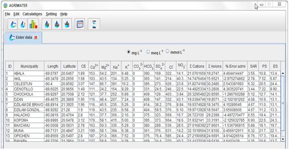
Inputting the data into the software, converting the units and storing the information produced in the database are processed that are performed in parallel. By selecting the units of the data and entering the interface “enter data”, the software automatically converts the quantity of ions into the following units: mg L−1, meq L−1, mmol L−1. Clinking on the “save” button saves the information, as shown in Figure 1. This procedure makes it possible to calculate water quality indexes, classify water types according to the Piper diagram, and to classify water quality according to the diagram of salinity and sodicity for n samples stored in the software database.
Calculation of indexes
The calculation of the indexes of water quality (SAR, PS, ES), the summation of cations and anions and the estimation of the percentage of allowable errors are done through the “edit” interface. The user needs only to select the option “modify”, click on the desired station and then click on the “calculate” button; the software will automatically recalculate the new indexes, the percentage of allowable errors and the summations, showing the new values in the table and saving them to the database, as shown in Figure 1.
To estimate the permissible levels of the water quality indexes of a certain station, it is only necessary to click on any value of the indexes, and the software will automatically display a graph that shows the evaluation of water quality with different colors: a) the bar is green when the level is low; b) the bar is yellow when the level is conditioned; and c) the bar is red when the level is not recommended.
Graphical methods
The graph interface is very simple. By rightclicking the desired station, it is possible to determine the chloride concentration of the sample and graph the levels of the major ions. The graph can be exported to a .png or .jpg file.
Water types are classified using triangular diagrams representing the proportion of three components in a set or a substance (Piper 1944). The Piper diagram represents the classification of water types as a function of the concentrations of the major ions. This diagram consists of two triangles and a rhombus; the left triangle indicates the cations; the right triangle indicates the anions, and the rhombus in the center represents the classification of water types. In the direction of the arrows of the diagram, each vertex represents from 0% to 100% of the concentration of a certain ion, as shown in Figure 2. To determine the concentration of cations based on the Mg2+, Ca2+ and (Na+ + K+) ions, it is necessary to convert the concentration values of these ions to meq L−1. Usually, the sum of the values is not 100%, and is thus necessary to determine the proportion of each ion, example:
Ca2+ = 7.66 meq L−1; (Na+ + K+) = 8.94 meq L−1; Mg2+ = 4.46 meq L−1
Sum of cations = 21.06 meq L−1
Percentage of
Similarly, we get (Na+ + K+) = 42.45% and Mg2+ = 21.18%

This gives the concentration of cations as percentages. Now a point is plotted in the triangle of the cations where all the concentrations intersect, and the procedure is repeated in the triangle of the anions Cl−, SO2−, (HCO− + CO2−). This gives the concentration of cations and anions in the water sample.
The classification of water types is based on the intersection of the points indicating cations and anions within the rhombus, which is divided into four regions: a) chlorinated and/or calcium sulfate water, represented in red; b) sulfated and/or calcium chlorinated and/or magnesium water, shown in gray; c) sodium bicarbonate water, shown in green; d) calcium bicarbonate and/or magnesium water. The results of the classification can be exported in tabular format to an .xls file.
The diagram of salinity and sodicity allows to define the type of water suitable for different crops. Four classes of salinization risk and four classes of sodification risk were defined, resulting in 16 types of water (C1-S1, C1-S2, etc.), each of which requires different conditions to be used as irrigation wa ter (Silva et al. 2013).
The diagram interface allows to: a) determine the proportion of pixels corresponding to the sodium absorption ratio in the y-axis, (values 0 to 30); b) determine the proportion of pixels corresponding to electrical conductivity in the x-axis (values 0 to 5.0); c) plot a point on the intersection of the values of sodium absorption ratio and electrical conductivity, repeating the procedure for each of the samples stored in the software database; d) identify the section of the diagram where the points were plotted and assign the corresponding class to each of the samples. The results of the classification are displayed in tabular format, which can be easily exported to an .xls file, as shown in Figure 3.

Changes over time
The trend analysis interface uses MK and TS tests to identify upward and downward trends for each of the major ions in the water samples from each of the stations stored in the software, providing the following information in tabular format: identifier, parameter, number of elements analyzed, number of changes occurred and the numerical value of the test. In the MK test, a value of Z higher than the threshold of 1.96 indicates an upward trend; if it is lower than -1.96, it indicates a downward trend. In the Sen’s test, a positive value indicates an upward trend; if the value is negative, it indicates a downward trend of the parameter or the index.
In northern Mexico arid and semiarid climates predominate; in the center and south of the country there are several months with little or no rain and, in addition, with the presence of the heat wave (Delgado et al. 2017; Montiel et al. 2019). This situation causes that both climate drought and seasonal drought are elements of the environment that involve the use of irrigation water and / or the selection of drought-tolerant crops (Delgado et al. 2010, Silva et al. 2013, López-Hernández et al. 2018; Ortega et al. 2019). This situation leads to many meticulous studies of the quality of water, both underground and surface bodies (Rubio et al. 2014, Almazán-Juárez et al. 2016). In this sense, the Agriwater software becomes a useful tool for quickly and efficiently calculating salinity indices, including those of potential salinity and effective salinity that are very often not taken into account (Delgado et al. 2010).
The Agriwater software performs most of the functions performed by other commercial software such as Aquachem (Table 1) (WH 2020), but Agriwater is focused exclusively on the evaluation of quality of water used for agricultural irrigation and does not intend to perform other types of analysis. The main advantages of Agriwater are that it can run on any operating system, its user-friendly interface that makes it easy to interpret the results and that it can be used in english and/or spanish.
Table 1 Properties and functions of Agriwater and AquaChem
| Properties and functions of the software | Agriwater | AquaChem |
| 1 English and/or Spanish as operating languages | Yes | No |
| 2 Data persistence (database) | Yes | Yes |
| 3 Multiplatform (Java) | Yes | No |
| 4 User-friendly interface | Yes | No |
| 5 Simple and easy analysis of water quality data | Yes | Yes |
| 6 More than 25 types of graphs | No | Yes |
| 7 Automatic calculations of water types, quantity of anions and cations, unit conversion | Yes | Yes |
| 8 Calculation of descriptive statistics | Yes | Yes |
| 9 Water quality based on official standards | No | Yes |
| 10 The data can be exported | Yes | Yes |
| 11 Geochemical modeling with PHREEQC | No | Yes |
| 12 Trend Analysis | Yes | Yes |
| 13 Alert levels | Yes | Yes |
| 14 Generation of automated reports | No | Yes |
The Agriwater software is a new professional tool that allows users to organize, store and process large amounts of data of the chemical composition of water in a simple, fast and accurate way. The Agriwater software improves the following processes: a) managing data of the quality water from hundreds of wells; b) converting units to improve data management; c) calculating various indexes of water quality for irrigation; d) evaluating water salinity and sodicity to avoid contaminating the soil; e) evaluating the toxicity of soluble ions in crops to improve agricultural production; f) identifying the type of water based on the percentage of ions, which allows for a better understanding of the effects of water on the soil; g) evaluating the changes in the quality of irrigation water over time to prevent the degradation of agricultural soils. In addition, the graphical interface of the software allows the user to operate it with ease and to interpret the results at a glance

