


 nova página do texto(beta)
 Inglês (pdf)
 Artigo em XML
 Referências do artigo
 Enviar este artigo por email
 Citado por SciELO
  Similares em
SciELO
Similares em
SciELO 
 Permalink
INTRODUCTION
Flow discharge and hydrodynamic measurements of any aquatic system allow us to know that habitat and, at the same time, analyze how it can be altered from an environmental point of view. Currently, these variables are measured using acoustic Doppler equipments, also known as acoustic Doppler current profilers (ADCPs) (Winterwerp et al. 2006). ADCPs have become popular due to their efficiency, speed and quality in flow measurement (Szupiany et al. 2007, Priego-Hernández and Rivera-Trejo 2016). They use frequencies greater than 25 kHz, which allows them to quantify the vibration of particles suspended in water. At a low frequency, the amplitude of vibration is equal to that of the medium, but the increase augments the effect of the inertia of the particles. At frequencies greater than 25 kHz, the vibration remains stationary, allowing the flow velocity to be measured (Vogt and Neubauer 1976). The ADCPs, depending on their configuration, work at high or low frequencies, and even with the combination of the two; this determines the range, penetration and number of cells (discretization) of the acoustic pulse in the water column. Another feature of ADCPs is their difficulty in measuring velocities close to the bottom of the channel (Simpson 2001), which translates into error (Fulford and Sauer 1986).
The measurement error of velocities measured with an ADCP is of the order of ± cm-1. In measuring the flow of a river with different ADCP configurations, Mueller (2002) found that they had a difference of the order of ± 5%. Currently, ADCPs are used for the quantification of sediment transport (Venditti et al., 2016), detection of secondary currents (Priego-Hernández and Rivera-Trejo 2016), monitoring of wetlands (Arega 2013), understanding fluvial habitats (Cundy et al. 2007), knowledge of aquatic ecosystems (Chang et al., 2015) and calibration of numerical models (García-Reyes et al. 2017).
For all the aforementioned reasons, it is important to select the ideal or most suitable equipment. However, it is common to find equipment that has different configurations (operating frequencies), which measure the same depth range. Given this situation, there is uncertainty about the type and quality of data obtained with each device. Therefore, the aim of the study was to compare the use of three acoustic Doppler current profilers that operate at different frequencies (2 000 kHz, 1 500 kHz and 600 kHz) in the Carrizal River and determine the most suitable equipment.
MATERIALS AND METHODS
The study was carried out in the flood season in a section of the Carrizal River, located near the capital of the state of Tabasco, Mexico (Figure 1), in zone 15 N of the Grijalva hydrological region, Usumacinta (RH-30), Grijalva subbasin, Villahermosa (RH-30Dv). The river is one of the most important in Southeast Mexico; the selected section has a low sinuosity (sinuosity = 1.27), no obstacles and constant area. The flow regime is classified as subcritical (plain river), with an average slope of 0.0003 measured from the El Macayo gate to the Grijalva-Carrizal confluence. It has an average annual flow rate of 350 m3 s-1, with a maximum annual flow rate of 1 466 m3 s-1 (Rivera et al. 2010).
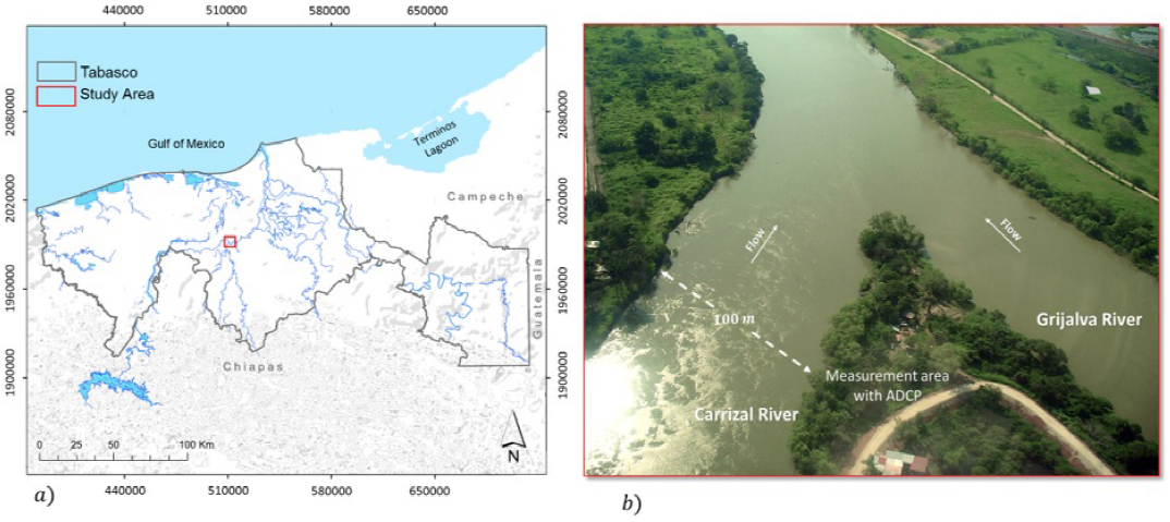
Figure 1 a) Location of the Carrizal River in the state of Tabasco, Mexico b) Measurement point in the Carrizal River.
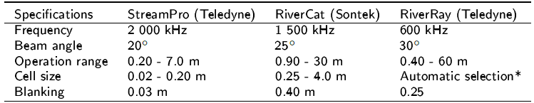
Three acoustic Doppler current profilers (Table 1) that work at the following frequencies were used: 1) 2 000 kHz, 2) 1 500 kHz, and 3) 600 kHz. Measurements were made in an approximately 100-m-wide cross section; five trips or measurements were made with each of the ADCPs mounted on a motorboat. Each trip took approximately 5 min, starting from the left riverbank and going to the right one as suggested by Pérez and Diaz (2000). The size configurations of the ADCP measurement cell were 0.20 m for the 2 000-kHz ADCP and 0.50 m for the 1 500-kHz one, whereas the 600-kHz ADCP was auto-configured every 0.10 m in the first five cells and 0.40 m in the remaining cells until reaching the total measurement depth, which was of the order of 5 m. The data obtained with the three ADCPs in the cross section were captured with the equipment's operating software (River Surveyor® or Winriver II®). With the data, a spreadsheet was generated in Excel® to perform the filtering to classify the data according to: 1) flow velocity components, 2) measurement depth of each vector, 3) measured transversal distance between each vector, 4) total distance of the cross section and 5) geographical position of each velocity vector. Then the velocity field graphics were constructed with the Tecplot® software.
Equipment calibration
It is essential that the velocity vectors be measured in the correct direction, so the internal compass of each equipment must be calibrated before the measurements, a process known as Heading, Pitch and Roll (HPR). The calibration for the 2 000 kHz and 600-kHz ADCPs was made with circular movements on their horizontal plane in the clockwise direction, while in the 1 500-kHz equipment the circular movements were made on the vertical plane. Magnetic declination is a variable that must be supplied to the equipment, depends on the coordinates of the study site, and is calculated as the angular difference between the magnetic North Pole and the geographic North Pole. The magnetic declination was obtained from the British Geological Survey webpage (BGS 2015). Another parameter to be taken into account is the mobility of the river bottom, which was determined by leaving the vessel stationary and then measuring it with each ADCP for 5 min. This is because the ADCPs detect whether the bottom is mobile, and, if so, the software corrects the measurements automatically.
RESULTS
Velocity fields and planform maps of velocity vectors
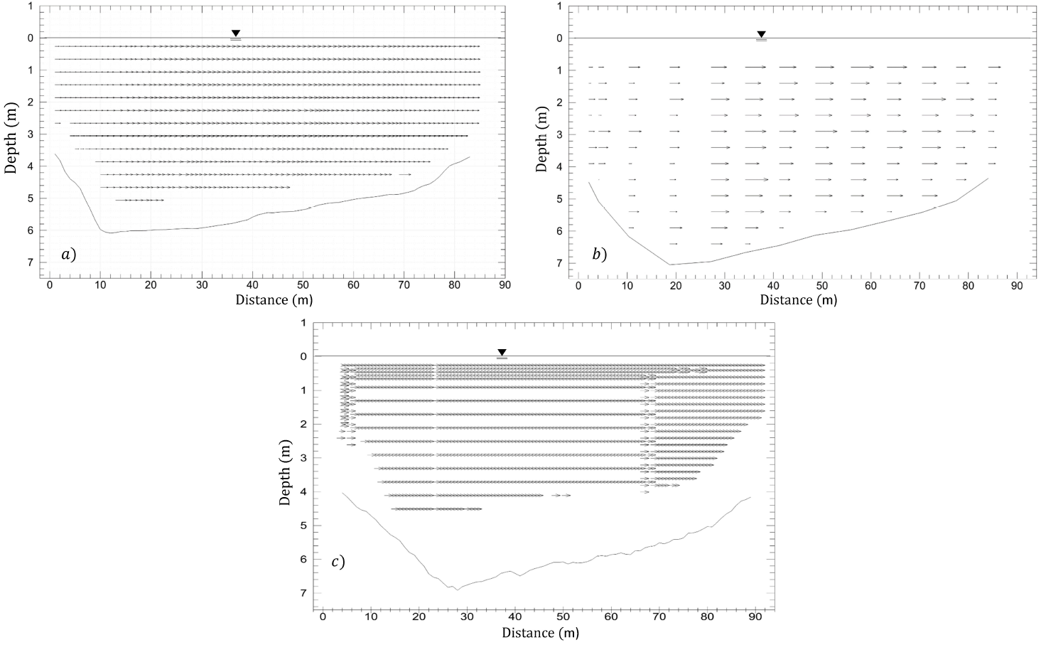
Figure 2 shows the magnitudes of the velocity fields measured in the cross section, with each of the acoustic profilers. It can be seen that the smaller magnitudes, in blue, are at the banks, while the larger magnitudes, in red, are located in the center of the section. One can also see the size of the blanking zones, without measurement, where the velocities of the bed near the channel and the banks cannot be quantified with the ADCPs. In Figure 3a-c, (b) the planform maps of velocity vectors of each ADCP are plotted, showing the flow path or current lines, measured in the cross section under study. These results can be combined to superimpose other phenomena, such as sediment transport or pollutant dispersal. Also in Figure 3d the comparison between the planform maps of velocity vectors measured with each ADCP is observed. It can be observed that the 1 500-kHz ADCP presented deviation in its path, due to the direction the vessel followed. Therefore, repeating the measurement at least five times is recommended, since comparisons are made with the average value.
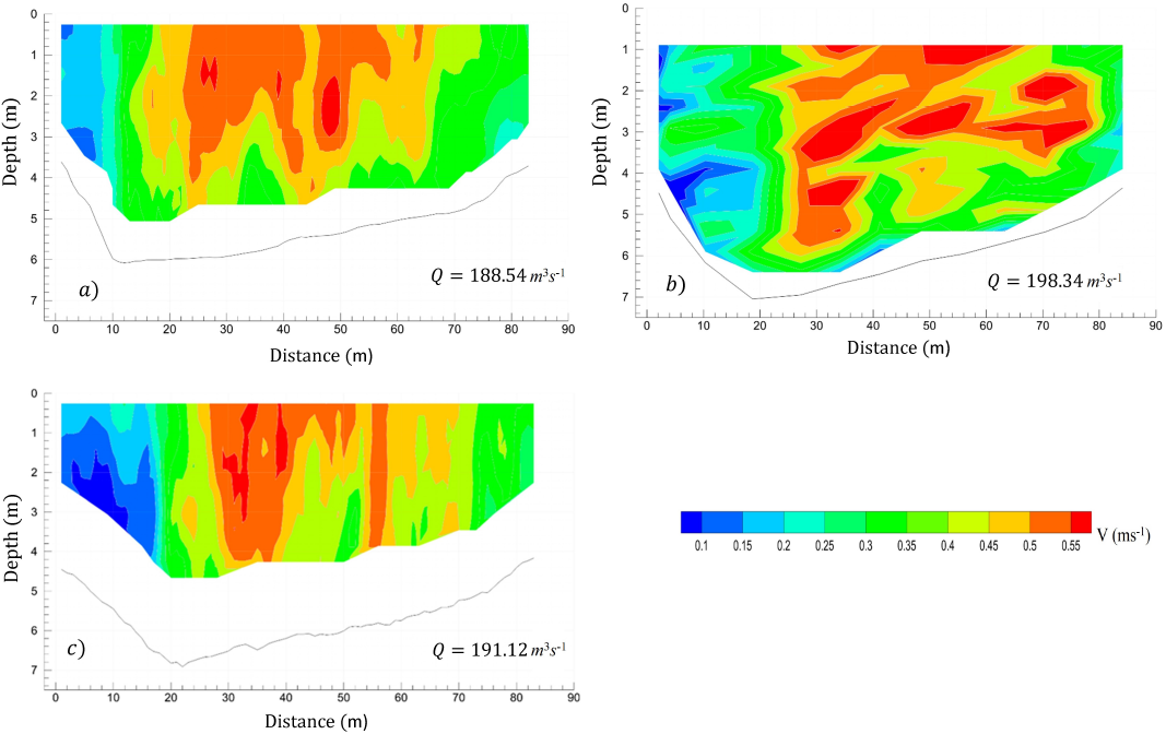
Figure 2 Magnitude of the velocity vectors in the cross section: a) 2 000 kHz; b) 1 500 kHz; c). 600 kHz.
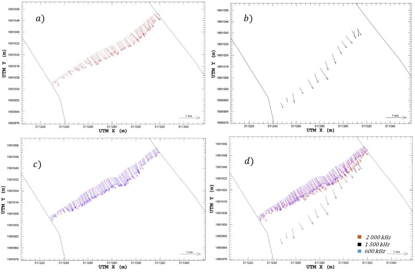
Figure 3 Planform maps of velocity vectors a) 2 000 kHz; b) 1 500 kHz; c) 600 kHz and d) comparison.
In Figure 4 it can be seen that for a depth of up to 5 m, the 2 000-kHz ADCP has a more detailed velocity distribution, arrows closer together, compared to the other two devices. This same Figure also shows that the 1 500-kHz ADCP has greater spacing between the velocity vectors and a blanking zone of approximately 0.90 m. It can also be seen that the 600-kHz ADCP has greater detail in the first 0.50 m, because the size of its cells is smaller; however, after that depth the size grows and the vectors also have greater separation.
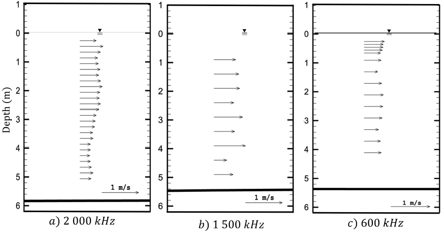
Table 2 shows the average values of the velocity magnitude in the water column of the cross section studied. The separation between the measurement depths of each device, which is a function of the cell size used, can be seen. Table 3 presents the flow measured with each ADCP in the cross section. The standard deviation associated with the flows obtained with the 2 000-kHz ADCP shows a small variation, when compared with the flow rates obtained with the 1 500-kHz ADCP, which has a higher standard deviation. Table 4 shows that the highest number of cells per unit area was obtained by the 2 000-kHz ADCP, which is explained by the equipment's cell size of 0.20 m and measuring time of 1.40 s. When comparing it to the 0.50 m cell size of the 1 500-kHz ADCP, it has a smaller number of cells per unit area with an equipment set time of 4.57 s, which implies that the transducer software will seek to interpolate the data where the ADCP cannot measure, which increases measurement error.
Table 2 Number of cells and velocity magnitude at points in the water column.
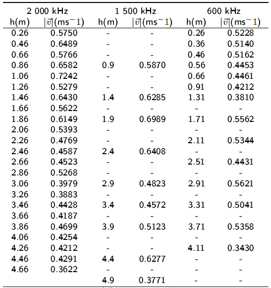
h, measurement depth;
Table 3 Average flow rate in the cross section under study.
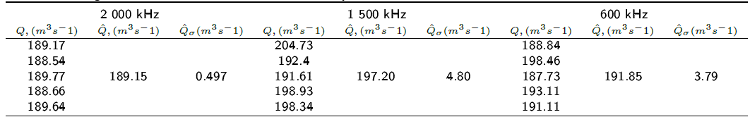
Q, instantaneous flow rate;

DISCUSSION
Table 3 shows that the 1 500-kHz ADCP had the highest uncertainty, approximately 5%, which coincides with Mueller (2002), while the 2 000-kHz ADCP had the least uncertainty. The flow velocity magnitude results obtained by the three ADCPs (Figure 2) differ in the distribution of the color range, because it corresponds to field measurements. The three ADCPs showed that the highest velocities are in the center of the river's cross section. This is a common finding in the cross section of a straight stretch of river with no obstacles, and these velocities coincide with what was found in previous studies (Baranya et al. 2015, Riley and Rhoads 2011). In the case of velocity profiles (Figure 5), the best distribution was with the 2 000-kHz ADCP, the values of which are more discretized or with a greater number of cells, in the vertical and horizontal scales. These results contrast with those obtained with the 1 500-kHz and 600-kHz ADCPs, which despite having a greater and smaller number of measurement points respectively, the distribution of their velocity profiles does not improve the quality. Regarding Szupiany et al. (2009) and Baranya et al. (2015), they indicate that a more uniform distribution in the velocity profiles allows for a detailed visualization of the transversal or secondary velocities. In addition, based on the velocity profiles, tangential stresses on the river bottom and Manning's roughness coefficients are determined and related to the suspension and bed load sediment transport. In this regard, in the present study, the best distribution was with the 2 000-kHz ADCP. Regarding Szupiany et al. (2009) y Latosinski et al. (2014), they developed several methodologies to estimate suspended sediment transport from measurements with Doppler equipment, without reporting difficulties or limitations of the equipment. This work corroborates the results of Mueller et al. (2009), who indicate that high turbulence and high bed sediment transport cause measurement problems in the ADCP. This is more noticeable in high-frequency equipment, where the wavelength is very small, with acoustic energy losses due to absorption of suspended sediments of the return beam, so that the signal can be lost or distorted at depths greater than 5 m on the other hand, profilers that work at low frequencies have more penetration power, which allows solving this limitation. An additional advantage of using an ADCP, when compared to measurements made with mechanical current meters, is the measurement time (Muste and Spasojevic 2004). For a mechanical current meters, about one or two hours are needed to perform the measurements, while with an ADCP the process takes an average of 15 minutes. The only disadvantage that ADCPs have, in addition to their cost, is that their use is complicated and the operator must be trained in its configuration, measurement techniques and data processing.
CONCLUSIONS
Comparisons among the 2 000-, 1 500- and 600-kHz ADCPs show that choosing the correct frequency is essential for selecting the measurement equipment. For flow discharges, any frequency is useful, as long as the equipment is in its operating range; however, to describe the structure of the flow, the best ADCPs are those that work at high frequencies, such as the 2 000-kHz device, taking into account that the higher the frequency the lower the penetration power in the water column.

