


 nueva página del texto (beta)
 Inglés (pdf)
 Artículo en XML
 Referencias del artículo
 Enviar artículo por email
 Citado por SciELO
  Similares en
SciELO
Similares en
SciELO 
 Permalink
INTRODUCTION
Income inequality has always been a very important topic among social scientists, but nowadays it also has an important place in the political agenda in many countries around the world. New governments came to power with the motto of decreasing income inequality through several re-distributional policies. In Mexico a new left-leaned political party came to power in 2018 and began to address income inequality since the very first day in office. This work is an attempt to provide a picture of the state of income inequality at municipality level, using the official statistics of Mexico. The main objective is to provide detailed measures and the possible causal relations among several explanatory variables such as federal grants.
This work is organized in four parts. This first is an introduction with a literature review on income inequality in Mexico. The second part contains estimation of the Gini and Atkinson indexes. These measures were constructed using microdata from the Mexican Inter-census Survey 2015 by the Instituto Nacional de Estadística y Geografía [National Institute of Statistics and Geography] (Inegi). In the third part we include a hierarchical clustering analysis to observe differences in groups based on inequality, poverty and economic development variables, and we use the Gini index to run a weighted least squares regression and analyzing the effect of federal grants authorized to the Mexican municipalities. The last part of this work summarizes the results.
LITERATURE REVIEW
Income distribution measurement is an important part of any normative analysis, and any change in the distribution must be assessed properly when making public policy. An extensive treatise on income distribution measures can be found in Allison (1978), Atkinson (1970) and Cowell (2000). All of them explain the advantages and disadvantages of each measure and compare many of them in terms of different benchmarks. Among the most efficient measures are the well-known Gini index and the welfare-based Atkinson index, which are the focus of this work.
In recent years there have been several new works focused on income inequality, some of them have been best sellers like Piketty (2015) which have increased the interest on the subject. Piketty and Saez (2003; 2014) are also works of the same author warning about the increasing income inequality in modern times. Bourguignon and Fields (1990) and Bourguignon (2004) are two works that contribute to the debate on increasing income inequality and the problem of poverty. They are intended to draw a relationship between these two issues and to alert of the danger of more divided societies.
Feldstein (1998) argued on favor of a redistribution policy based on poverty reduction rather than reducing income inequality. In terms of welfare, he convincingly argued that it is not wrong that rich people get richer as long as poor people is not affected. This is perfectly in line with Pareto Welfare theorems that many economists embrace in their welfare analysis. Perhaps as a coincidence, during this time Mexico constructed redistribution policies based on solely poverty alleviation. Currently most Mexican official social programs, including federal transfers to local government, are designed with the objective of reducing poverty.
One important first attempt to explain the causes of income inequality is Garvy (1952). He outlined the factors that determine the personal incomes:
Endowments: both, inborn and abilities acquired by learning, along with inherited physical capital and advantageous environment.
Economic cycles and growth.
Redistribution policies by the Government.
Demographic and labor market factors.
Geography and urbanization.
Income distribution over time compared with all other factors.
But perhaps one of the most influential works of our time is Sen (1999), which is a strong critique to the neoclassical theory of distribution, including the Rawlsian view of distributive justice. He introduces the concept of “capabilities” in a framework of justice and “functionings”, and offers a view of the factors that make more unjust the relation between real income and actual disadvantages among individuals. Summarizing, he pointed out five sources of such disparity as:
Individual heterogeneity and physical differences such as gender, age, physical disabilities, etc.
Environmental differences such as climate, pollution, exposure to deceases, etc.
Social stability and social capital, such as social infrastructure, violence, crime, wars, etc.
Differences in relational perspective such as social conventions, customs, discrimination, religion, etc.
Distribution within family.
In Sen’s view, individuals with these disadvantages have less command and control of their resources at their disposition. Because of these, their capacity to function is limited and then any redistribution will be of limited improvement.
Recently, other important thinkers also explore the reasons for perpetuating income inequality and Heckman (2011) is just an example of this. He has written extensively in the effect of early childhood education and its effects on life time income and inequality. In this thinking, he suggests investing in education early in life so that to increase the returns of such investment and then life time income.
But we cannot neglect the effect of macroeconomic policy, real cycles, fiscal policies, regional and urban development even the effects of geographic factors and distribution of natural resources. For example, Esquivel (2000) is a work that explains that climate and vegetation determines the differences in per capita income by regions in Mexico. He offers some evidence that geography has an important role in the distribution of income.
Perry et al. (2006) is an excellent work that debates on the relationship between economic growth and poverty. They compare economic growth and poverty reduction in developed countries with the performance in Latin America in recent years. They analyze how both phenomena reinforce each other, but still support the thesis that growth reduces poverty although poverty may have an effect of delaying economic growth.
Bárcena et al. (2018) is an economic report on Latin America and deals mainly with economic inequalities (means, opportunities, capabilities and acknowledgement) and the idea that these inequalities induce high economic costs that hinge economic growth and development.
Another important variable are federal transfers, which are perhaps our scientific aim in this paper. Some authors believe that direct transfers to families have contributed positively to decrease income inequality. Because federal grants are designed with a specific formula that includes poverty parameters, there is a direct relation between them, but the relationship between federal grants and inequality is little understood at local level though we assume that poverty and income inequality are strongly correlated.
Since 1990s federal transfers are an important part of the fiscal system in Mexico, representing about 80% of local (municipal) revenue. Mexican fiscal system concentrates most of the tax revenue and allocate resources to local governments according with two broad principles: tax effort and redistribution. The general-purpose federal transfers referred as Participaciones federales also known as Ramo 28 compensate for the tax effort at local level, giving back to each state and municipality the revenues needed for operational activities. The conditional grants called Aportaciones federales, also commonly known as Ramo 33, are designed to improve fiscal position and are specific grants which must be invested in social programs and local public investment. The funds allocated in the Ramo 33 are designed strictly to increase and improve the provision of local public goods and services. So, it is expected that local governments with high levels of poverty and under-provision of local public goods may receive relatively more than richer local communities and the reverse is for Ramo 28.
Angeles, Salazar and Sandoval (2013; 2019) are two works that research on the effect of conditional grants on inequality. Both works analyze the effect of conditional grants on economic growth, inter-state per capita income gaps and income inequality within each Mexican state. They use state level data and perform panel analysis. In the first work they found no robust results that can explain the effect of conditional grants on income inequality, only a decline in the long term. In the second, they concluded that conditional grants do not improve income inequality within each state. They also found robust results that income gaps among states increases with conditional grants. Although these works are illustrative, they use aggregate data, which may dilute some important details that can be observed with a smaller political entity.
The consensus among researchers is that income inequality in Mexico has decreased in the last three decades at least, and mainly due to government transfers to families through social programs. Campos, Esquivel and Lustig (2014) and Scott (2008) both agree that income inequality has decreased due to the several government transfers such as Progresa program and other grants to rural families, health institutes and pensions. Then, we also want to complement the literature on this topic, analyzing regional and local disparities and the effect of conditional grants on such disparities.
METHODOLOGY
Gini and Atkinson indexes
In this section we introduce an estimation of the municipal Gini and Atkinson indexes for Mexico. The Gini and Atkinson indexes were constructed using data from the Mexican Inter-Census survey 2015, from the Inegi (2015), the same data used by the Consejo Nacional de la Evaluación de la Política de Desarrollo Social [National Council for the Evaluation of Social Development Policy] (Coneval) (2018) to calculate the multidimensional poverty index. The data sample is representative to municipal level and collected by dwellings rather than households. We consider the concept of extended household to interpret the information on each dwelling, as it is custom for some families to share the same dwelling with other close family members, though this is not a widespread practice.
The Mexican Inter-Census survey 2015 has a sample of 6.7 million households for a total of 2,446 municipalities.1 The average sample was 2,722 households per municipality though the minimum was 7 and the maximum municipal sample was 40,203. There were no data for 11 municipalities and 398 municipalities did not report information on federal grants.
The whole data set was collapsed in each household in order to add up the total income for all household members. We equate household as the same as extended family, accepting that at least some generations may share the same roof and part of their income. This is not completely unrealistic because many households in Mexico hedge different risks through family bonds. The lack of universal social security, inefficient labor markets and incomplete insurance markets are the main problems that many Mexican households face either in the urban slums or rural regions. So, in this work we treat dwellings and (extended) households as the same.
The Gini index is a well know income distribution measure and can be defined as
the shaded part of the Lorenz curve. A simple and general formula can be
constructed if we define the Lorenz curve as
On the other hand, the Atkinson index is based on the idea of a social welfare function. Let us assume a utilitarian welfare function as:
Where there are as many as i individuals. Let us assume that each individual utility function is in the form:
Where
Substituting the utility function in the Welfare function, and equating with ye we define:
The Atkinson index is defined as:
Where
Cluster analysis
We also produce a cluster analysis of income inequality using some socioeconomic and fiscal features. The main idea is to classify municipalities according to income inequality measures and other characteristics, such as mean income, population, poverty and marginality, government transfers and other social and urban factors such as education, health and sanitation.
The main objective is to find a pattern that can explain the spatial distribution according to income distribution measures along with poverty and marginality. If we could obtain a classification from the data, then we might be able to establish possible relationships between income inequality and other features. There are already some classifications in terms of poverty, marginality and social lag, all constructed by government agencies. But we want to construct a classification based on patterns produced by the dataset itself. So, we decided to construct a dataset with several variables that may describe disadvantageous conditions in each municipality, such as income inequality, poverty, education, health levels, etc.
A natural way to classify data may be the use of machine learning methods, and
perhaps clustering analysis is a very convenient simple algorithm that does not
require supervision. The nearest neighbor algorithm is the simple way to classify
data and determine how close (far) is a point in Rn space is from other
points. We can use the Euclidean distance
The Human Development Index (HDI), with its health and education indexes, were obtained in the Programa de las Naciones Unidas para el Desarrollo [United Nations Development Program] (PNUD) (2019). The fiscal, demographic, urbanization came from the municipal data base of Inegi (2015).
Regression analysis
Another part of our analysis is to explore the relationship between income inequality and possible effects from the federal grants to municipalities in per capita terms, in special those conditional grants designed to reduce poverty. These grants can also be considered direct grants to households because there are used for local public goods and services. A regression model was constructed, using the Gini as the dependent variable:
The explanatory variable Y is the log of the mean household income in municipality i, the vector of federal grants is T and a vector of other socio-demographic variables are included in S. Federal grants are divided into conditional and unconditional grants. Among the economic development variables used the education and health indexes used in the calculation of the HDI. We also added a sewage index for taking into account the degree of urbanization.
One problem we might face in our regression analysis is endogeneity. We decided to perform a Two Stages Least Squares (TSLS) regression, and used instruments to estimate the variable of log mean household income. Because we are dealing with the mean household income by municipality, this might be affected by the development conditions. In order to correct for heteroscedasticity we run instrumental variables regression with robust standard errors.
RESULTS
A map in figure 1 shows the Mexican territory divided by municipalities, colored using six levels of Gini. The darker has the highest in income inequality, and we can see that southern states such as Oaxaca, Guerrero and Chiapas have high income inequality, but also some parts of Durango, Chihuahua, among other regions. On the other hand, the map in figure 2 shows a multidimensional poverty index designed by the Coneval. Comparing both maps we may see that poverty is concentrated in the center and the south of Mexico, while the Gini and therefore Atkinson measures are more dispersed along the country, though the darkest areas are pretty similar2 which may imply correlation.

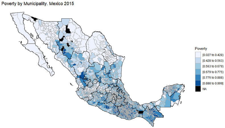
Source: Author’s elaboration with the Coneval data.
Figure 2 Multidimensional poverty in Mexico, 2015
As mentioned before, poverty is the main policy objective in Mexico when formulating redistributive policies. Some official indexes have been constructed so that to help implementing poverty alleviation programs such as Progresa and Oportunidades. Most scholars and international institutions agree that these programs have been successful in reducing poverty. For example, Lustig, Lopez-Calva and Ortiz (2012) and Lopez et al. (2012) report that poverty and income inequality decreased due to these government transfers; and Gantner (2007), also agree that poverty alleviation policies in Mexico have been successful.
Although poverty and income inequality have been decreasing in the last decades, we also need to know about the spatial configuration of such income inequality and poverty patterns. We want to observe if poverty alleviation policies have also reduced inequality. We want to know if those geographical areas considered poor have similar levels of income inequality. Defining a poverty line is somehow insufficient for classifying those people with social disadvantage. On the other hand, a measure of income inequality clearly exposes the disparities and disadvantages within a community or country. Although income is not a perfect measure of economic progress, its distribution can tell us on the relative disadvantage an individual has, related to others with more command on goods and services they need to function. We expect that redistribution policies also reduced the gap between poor and rich. So, we want to corroborate this assertion.
Clustering analysis is convenient to visualize data, so we can construct a dendrogram which is a tree graph like. We are looking for features that allow association in the data, so we expect some correlation. But correlation itself cannot be the only criteria used to select our features. Using the standard literature, we decided to begin our variable selection by choosing proxies of demographic, geographic, economic and social variables related to disparities in household income. Chart 1 contains the Pearson correlation for all chosen features.

After selecting our variables, we normalized our data set to avoid undue influence of large metrics. The dendrogram produced by hierarchical clustering using complete linkage can be seen in chart 2. This tree graph shows two large subgroups that can be classified as municipalities with high and low-income inequality. High income inequality municipalities are a special case and of major interest in our research. Both groups can also be divided into two subgroups that we may call medium-high and medium-low income inequality. Hierarchical clustering is non-supervised classifier that relates objects according with their similarities (closeness) to each other. The selection of these groups and subgroups is decided to keep homogeneity without being too general. We are especially interested in the high-income inequality subgroups as those supposedly contain the majority of municipalities classified as poor or marginalized.

Using the hierarchical clustering, we decided to classify all the 2 446 Mexican municipalities into four large groups: low-income inequality with 551 municipalities, 1464 municipalities as medium-low income inequality and another 169 considered medium-high income inequality and finally a high-income inequality group with 262 municipalities. Table 1 shows a table of statistics representing some average values classifying by these groups and for some important features associated with each subgroup of municipalities. In terms of income, we observe that municipalities with high mean income usually have lower income inequality. But for the high inequality group the average population is less than the middle-high inequality group. This reversal can be observed also in the percentage of sewage systems, matching grants, schooling, child mortality, poverty, social lag and marginality. There is evidence that there are municipalities with highest income inequality, but they are not the very poor ones or the more disadvantaged. The poorest municipalities in Mexico usually have moderately high-income inequality.
Table 1 Average features by inequality group 2015
| Income | ||||||
|---|---|---|---|---|---|---|
| Type inequality | Income | Log income | Population | Gini | Atkinson | Sewage % |
| Low | 9 376.01 | 9.10 | 143 010.74 | 0.42 | 0.15 | 0.96 |
| Medium-low | 5 369.54 | 8.52 | 25 006.00 | 0.47 | 0.22 | 0.84 |
| Medium-high | 2 921.98 | 7.91 | 7 090.01 | 0.58 | 0.38 | 0.31 |
| High | 2 752.66 | 7.68 | 10 556.65 | 0.70 | 0.54 | 0.68 |
| Fiscal features | ||||||
| Grants in current Mexican pesos (million) | Grants Per capita | |||||
| Type inequality | Conditional | Uncondi-tional | Deficit | Conditional | Uncondi-tional | Deficit |
| Low | 150.08 | 165.49 | 17.02 | 1 723.47 | 2 571.29 | 230.08 |
| Medium-low | 51.79 | 33.17 | 2.50 | 2 021.98 | 1 369.46 | 111.98 |
| Medium-high | 22.80 | 7.35 | 0.71 | 3 558.50 | 1 314.60 | 106.71 |
| High | 34.27 | 13.14 | 0.36 | 2 983.11 | 1 851.28 | 127.45 |
| Social features | ||||||
| Type inequality | Schooling | Child mortality | HDI | Poverty | Social lag | Margina-lity |
| Low | 7.87 | 12.94 | 0.73 | 0.36 | -1.01 | -1.11 |
| Medium-low | 5.51 | 16.84 | 0.64 | 0.69 | 0.01 | 0.09 |
| Medium-high | 3.67 | 27.21 | 0.53 | 0.92 | 1.81 | 1.44 |
| High | 4.19 | 19.91 | 0.57 | 0.88 | 0.92 | 0.89 |
Source: Author’s elaboration.
We are interested in income inequality and mean household income so that we can have a better understanding on how income inequality relates with the economic development. The literature relates income inequality measures to income as there is an empirical notion that the size of income is also a proxy for economic development. Kuznets (1995) pointed out that in early stages of development inequality seems to be increasing and for modern economies must be decreasing. Barro (2000) confirm Kuznets’ hypothesis using a cross section country analysis.
Another way to interpret table 1 is to make a tabloid graph in order to present each inequality group separately. In chart 3 we plotted all groups by Gini index and the mean household income. A regression line is added to each group to have a better view of the relation between the two variables. The results show that, as expected, inequality is lower the higher the income for all groups except for the low inequality group. For the low inequality group, there is a positive relation between inequality and mean income. In this case, the classical view that inequality is increasing in early stages of development is not strongly supported. For all groups except the low-income inequality group, there is a negative relationship between income inequality and income as a proxy of economic development. This may be a fair prediction, but the low inequality group seems to show a positive relationship. Municipalities with very high mean income show a relatively high-income inequality. Although highly productive and more developed local economies are less unequal compared with less developed municipalities, just for this group there seem to be an unusual relationship that must be studied with detail, especially when some are predominantly urban.
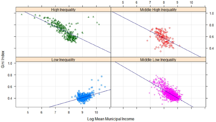
Source: Author’s elaboration.
Chart 3 Municipal income inequality and mean household income: by group
From the 157 municipalities with more than 150 thousand inhabitants, 136 are in
the group of low-income inequality. They represent the 66% of the total
population of Mexico, which also live in urban areas. This is an important, and
sometimes neglected fact, that people feel more unequal in large urban cities
where labor productivity gaps are more visible since inequality might be
increasing rather than decreasing. It is not difficult to link social unrest in
some parts of the world (including Latin America) where people with economic and
social disadvantages living in urban areas feel there are treated more unequal
or unfair. If we accept the usual assumption that, for example, human capital
grows at an exponential rate
For the high income inequality group the relationship is positive despite some extreme outliers.3 For medium inequality groups, the relationships are also positive between the inequality measure and mean municipal income. So, we expect that economic development may also decrease the income gap among individuals and households.
If we compare income distribution with other social indicators such as poverty, we see that there is a positive correlation between income inequality measures. Chart 4 shows the relation between Gini index and poverty index, using our classification of municipality by inequality groups. For all groups poverty and inequality measure are positively correlated, but for high income inequality group, the regression line is almost flat though still with positive slope. This graph is telling that there are little or almost no changes in inequality due to changes in poverty levels.

We know that the conditional grants provided to local governments are calculated using poverty and social lag as part of the equation. The Coneval provides to the Mexican congress with the parameters and rankings to be used in the design of the federal grants. Poor regions will receive relatively more conditional grants (Aportaciones federales) than rich ones. And vice versa, poor municipalities will receive less unconditional grants (Participaciones federales) than rich ones. This is the way fiscal policy is used for redistribution, which may reduce poverty and, in some degree, reduce income inequality. However, the effects on income redistribution through federal transfers may be limited or just nil inside the low inequality group. Poverty alleviation programs in rich, modern and urban clusters may have no effect on income distribution, then these programs may not alleviate any sense of separation or gap among households. To answer this question we are motivated to so some analysis on the effect of federal grants on income inequality.
We must also realize that income inequality is not only about income, but real access to economic opportunities and lifetime income returns. If only few get to accumulate faster and better, then the social web become more strained, especially in those geographically close communities where many types of households interact daily. Poverty is also strongly correlated with income, but if poverty is combined with inequality in rich municipalities, the social problems became more difficult to solve because the general sense of unfairness. What chart 5 is telling is that redistributing down to the poor, as the current federal budget is proclaiming, is not solving the social and economic gap among households.
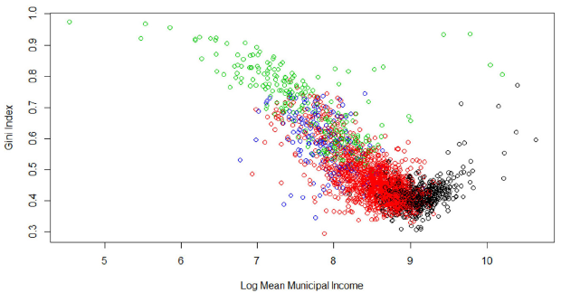
Source: Author’s elaboration.
Chart 5 Municipal income inequality and mean household income by groups
Economic growth with higher mean income will certainly reduce absolute poverty, but there is no guarantee that the income gap among household will be reduced, at least for some. For some Mexican living in large urban municipalities, income inequality may have not decreased by means of economic growth (higher income) and a better welfare state. Reducing poverty is a good goal for itself but cannot compensate for high levels of income inequality in some well-developed regions.
Regression analysis on income inequality
From the selected variables that may affect income inequality, we may try to perform additional statistical analysis in order to verify their relative influence. A severe problem of heteroscedasticity is present in the data, where the different subgroups have different variance with the only exception being the middle-high group. A white test was performed in order to check for this problem. A typical approach to eliminate this problem might be to do regression analysis with robust standard errors. Another problem is endogeneity and a Durbin-Wu-Hausman test was performed detecting endogeneity in the variable mean household income especially in the high and low income inequality groups. A TSLS regression was performed for each group using the Gini as the dependent variable and mean municipal household income in logarithms, conditional and unconditional grants as well as sewage, education and health indexes as regressors.
We already expressed some concerns about the group of low-income inequality. In our graphical analysis this group behaves different but only shows a positive relation between Gini and education and a negative relation between Gini and health. This group which happened to be mostly medium-large urban agglomerations shows a very distinct pattern of social and economic development compared with the other three groups. But, the regression analysis scarcely explains income inequality for low inequality group, and all federal grants do not appear to affect inequality at all. We also must notice that for this group the regression fit is also very low, with only an R2 of barely 0.025. The low income inequality group of municipalities seems to be the most complex with many more unobserved factors to be considered. Then, a more detailed analysis is needed to understand this group, perhaps studying separately urban and rural municipalities though we decided to pursue this analysis for future research.
Table 2 Two Stage Least Squares regression by group
| Gini | Low | Middle-Low | Middle-High+ | High | ||||
|---|---|---|---|---|---|---|---|---|
| Log Mean Income | -0.006 | -0.145 | *** | -0.128 | *** | -0.028 | ||
| (-0.0152) | (-0.0112) | (-0.0186) | (-0.0373) | |||||
| Log Conditional Grants | 0.005 | 0.012 | *** | 0.026 | 0.038 | ** | ||
| (-0.0034) | (-0.0039) | (-0.0157) | (-0.0152) | |||||
| Log Unconditional Grants | -0.0003 | -0.018 | *** | -0.029 | ** | -0.021 | ** | |
| (-0.0031) | (-0.0033) | (-0.0139) | (-0.0084) | |||||
| Sewage Index | 0.007 | -0.029 | ** | 0.024 | -0.131 | *** | ||
| (-0.054) | (-0.0128) | (-0.0363) | (-0.0315) | |||||
| Education Index (HDI) | 0.111 | *** | 0.087 | *** | 0.311 | *** | -0.115 | |
| (-0.0388) | (-0.0323) | (-0.108) | (-0.0979) | |||||
| Health Index (HDI) | -0.124 | *** | -0.048 | 0.055 | -0.081 | |||
| (-0.0427) | (-0.029) | (-0.0559) | (-0.100) | |||||
| C | 0.471 | *** | 1.754 | *** | 1.409 | *** | 0.969 | *** |
| (-0.130) | (-0.0941) | (-0.231) | (-0.316) | |||||
| Observations | 523 | 1,175 | 142 | 207 | ||||
| R-squared | 0.0250 | 0.5150 | 0.3330 | 0.440 |
Note: Instruments. Mean education level, population, marginality and social lag indexes and child mortality.
Coefficients show the estimation of the beta parameters.
The standard error is show in parentheses.
** Significant at .01. *** Significant at .001.
+ Middle-high group is a simple OLS regression as no endogeneity and heteroskedasticity detected.
Source: Author’s elaboration.
The group that is better explained by the regression analysis is the middle-low income inequality group which shows a negative coefficient in the mean municipal income. In this group, as municipalities improve in terms of economic growth and development, income inequality decreases. This relationship can also be observed in table 1 for middle-high income inequality group. So, we expect that it is true that economic development may decrease income inequality at some degree, so any policy directed to promote economic growth in this group will surely must be welcome.
Fiscal variables are also significant for medium-low income inequality municipalities. Conditional grants coefficient was positive and highly significant for high inequality and for medium-low inequality ones. The reason is that inequality is not the same as poverty, and because conditional grants were designed to reduce poverty, they might be negatively related to poverty but not to inequality. So, we expect that conditional grants increase income inequality for medium-low inequality. On the contrary, we can observe that unconditional grants decrease income inequality while they are not designed for this purpose.
The sewage and health indexes are significant and inversely related to inequality, which means that improvement in urbanization and health services decreases inequality, but urbanization decreases inequality for middle-low and high inequality groups while health services only improve income distribution for medium-low municipalities. Education index is significant but positive for all except the high inequality group, and the interpretation is that education increases inequality by making only some individuals highly productive while others do not benefit from human capital accumulation in the form of formal education.
For medium-high and high-income inequality municipalities only some variables were significant and can be interpreted in a similar way as for medium-low inequality ones. Unconditional grants reduce income inequality for both while conditional grants increase inequality for high inequality. Investment in urbanization is also a positive aspect for reducing inequality for the high inequality group.
Inequality vs social lag vs marginality
In this section we show the differences among official measures of poverty and marginality used to design social policy in Mexico with the classification we developed so far in this work. We believe that this analysis is important because it gives us information on the side of income inequality, a variable that cannot be neglected by policy makers when designing social policy.
Table 3 shows the number of municipalities described in terms of the official indexes such as social lag and marginality, but now related to a municipal classification in terms of income inequality. The information in this table is relevant because now we may observe which municipalities have the greatest social disadvantages but also have high income inequality. We already discussed that social and fiscal policy is designed at Federal level and aimed to reduce poverty. Social lag and marginality are two of the main indexes used to decide social investment and allocation of social goods. With this new classification we may also observe that some are classified with very high marginality and social lag have different levels of income inequality. For example, we know that there are 175 classified as very high social lag and 280 classified with very high marginality, but from those only 90 and 76 are classified as high income inequality respectively. We cannot discern which regions are priority in terms of allocation of grants and local public goods for low income recipients. On the other hand, we may observe that there are 15 municipalities considered with low social lag and 3 with social marginality but are classified as high income inequality.
Table 3 Classification of number municipalities with Inequality vs social lag and vs marginality
| Inequality | Social lag | |||||
| Very low | Low | Medium | High | Very high | Total | |
| Low | 303 | 238 | 10 | 0 | 0 | 551 |
| Medium-low | 38 | 507 | 523 | 362 | 34 | 1 464 |
| Medium-high | 0 | 0 | 1 | 78 | 90 | 169 |
| High | 0 | 15 | 69 | 127 | 51 | 262 |
| Total | 341 | 760 | 603 | 567 | 175 | 2 446 |
| Inequality | Marginality | |||||
| Very low | Low | Medium | High | Very high | Total | |
| Low | 297 | 213 | 36 | 5 | 0 | 551 |
| Medium-low | 48 | 279 | 444 | 586 | 107 | 1 464 |
| Medium-high | 0 | 0 | 3 | 69 | 97 | 169 |
| High | 0 | 3 | 31 | 152 | 76 | 262 |
| Total | 345 | 495 | 514 | 812 | 280 | 2 446 |
Source: Author’s elaboration.
This additional classification in terms of income distribution requires a multigoal social policy. We are confident that the concepts of poverty, social lag and marginality are multidimensional so household income is also included in these official indexes. Some may say that reducing poverty also reduces income inequality, but this is not entirely true. Poverty, social lag and marginality are heuristic concepts, and designed to set a cut-off line that can be used for redistribution. Those below a poverty line are subsidized and those above are not. But this policy only treats unfairly those just above the poverty line. Income inequality deals on how individuals are compared in terms of income which is affected by any transfer. Larger transfers may be required to bring a population out of poverty in a municipality with high income inequality than those with low inequality. So, they cannot be treated equality in terms of fiscal and social policy.
CONCLUSIONS
In this work we constructed a Gini and Atkinson indexes and compared them with other official measures of poverty. Although poverty is the main policy objective for many social programs, there is still consensus that many government transfers have had an overall positive effect in reducing income inequality in the last decades. But while studying income inequality with some more detail we observe that some Mexican regions are well developed but still suffering high levels of income inequality.
This paper offers some classification of income inequality based on clustering analysis, which is a non-supervised machine learning method. The classification of Mexican municipalities based on household income inequality was compared with those of official measures of poverty, marginality and social lag. We also performed some regression analysis using this inequality classification to observe some variables that affect income inequality by groups.
Our analysis shows there is a group of 551 municipalities that can be considered of very low income inequality where economic growth and development may be related to increases in inequality compared with the others. We also found that conditional grants designed to decrease poverty do not have any effect on this group.
On the other hand, conditional grants increase inequality for at least the middle-low and high income inequality groups while unconditional grants may have the opposite effect for all except for the low inequality group. These results support the idea that conditional Federal Transfers to Municipalities may deteriorate the income distribution while unconditional grants may help to improve the distribution of income despite this was not the main fiscal policy objective.
Income inequality compares how people is compared to others in the income distribution, while poverty only considers those below a threshold of multidimensional and variable needs. Despite the multidimensional poverty concept and for practical reasons, transfers are channeled to those in the bottom of the poverty scale, without considering their position in relations with others in the income scale. So, an inequality classification is also needed to contrast and consider a social policy with multi-objectives and priority regions based on other important factors such as income inequality. This topic is of such relevance especially in municipalities with low marginality or social lag with high income inequality, where the perception of social justice could be undermined. We are referring to those large municipalities with high income and high economic development but where inequality is relatively high.
In our analysis we were able to conclude that government grants may have an opposite effect on income inequality compared to poverty. Conditional grants are designed to reduce poverty but may be increasing income inequality at least for the medium low up to the very high inequality municipalities.
What this work is showing is that measuring social disadvantages is a complex business especially if we are dealing with a very heterogeneous population. Although official programs have improved the position of many families, the effect of such programs is different in every municipality and region in Mexico. The most obvious course of action may be to design poverty alleviation programs and income improving grants with a more multi-objective and measurable programs. Decreasing poverty and marginality are good aims for themselves but at the end, it is the perception of fairness and social justice that have an important role in promoting a more balance growth. And this perception is deeply rooted in income inequality.

