


 nueva página del texto (beta)
 Inglés (pdf)
 Artículo en XML
 Referencias del artículo
 Enviar artículo por email
 Citado por SciELO
  Similares en
SciELO
Similares en
SciELO 
 Permalink
The observation that species are not randomly distributed across the landscape but exhibit patterns to their distributions took shape as early as the 1700s, when Georges-Louis Leclerc (better known as Comte de Buffon) recognized that despite having similar environments, geographically disjunct regions bore different assemblages of plants and animals- today this is referred to as Buffon's Law of biogeography (Riddle 2017). Elucidating the determinants of species’ geographic distributions is a fundamental goal of ecology and biogeography, as these can provide insights that are relevant for key biological processes (such as adaptation) as well as for conservation in a time of rapidly changing environmental conditions (Sheth et al. 2020).
A species’ geographic range can be defined as a spatial projection of its realized ecological niche (Sexton et al. 2009), that is, the set of conditions where a species actually occurs and not just where it has the potential to occur given its physiological tolerances (fundamental ecological niche; Sexton et al. 2017). A species’ realized ecological niche encompasses everything from tolerances to abiotic factors to species interactions or biological aspects such as dispersal that can affect where a species can and does occur in nature. Beyond species’ tolerances, ranges can be shaped by key traits or biological interactions (both positive and negative). For example, in miner’s lettuce plants (Claytonia perfoliata, Portulacaceae), polyploids exhibit distinct and broader ecological niches than their diploid counterparts (McIntyre 2012). And, in plants of the genus Bromus (Poaceae), drought stress amelioration mediated by the association with mutualistic fungal endophytes facilitates their incursion into drier habitats and the broadening of their geographic ranges as much as 20 % (Afkhami et al. 2014).
Focusing on realized niche breadth integrates across historical and ecological factors and processes (including environmental filtering and species interactions) that could otherwise be ignored when analyzing fundamental niche breadths (which are themselves important when addressing aspects such as evolvability of adaptability, but typically require physiological estimates of tolerance). Key aspects of the realized niche are those related to the range of climatic conditions that species occupy, which can be expressed as climatic breadth or amplitude. Relationships between geographic distribution and climate are foundational to concepts of the niche (see review Holt 2009, Carscadden et al. 2020), going back to observations by Humboldt on altitudinal distributions of species and climate that predate the niche concept (von Humboldt & Bonpland 1807). In large part due to interest in understanding the implications of climate change, relationships between niche breadth and geographic range continue to be central in ecology (e.g., Rehfeldt et al. 1999, Slatyer et al. 2013, Carscadden et al. 2020).
Geographic range size conceptualized as a species trait, can provide insights about biological processes such as dispersal and adaptation (Sheth et al. 2020), which have consequences related to commoness and rarity, and thus to extinction risk and invasiveness potential. Thus, one key motivation to study the extent to which a species’ geographic range is associated with its niche breadth is that it might inform the level of a species’ susceptibility to changing conditions (Sheth et al. 2020). The ‘range size vulnerability hypothesis’ (Shay et al. 2021) postulates that species with narrow geographic ranges might be at a greater risk of extinction under changing environments, in part due to their likely smaller population sizes, but potentially also due to narrower physiological tolerances. Identifying such species by evaluating their range sizes and climatic breadths is one first important step for their conservation. It is also important to identify species that deviate from a general pattern. For example, species that despite having wide niche breadths still have restricted geographic ranges; or the converse, species that have large geographic ranges but exhibit narrow niche breadths and thus still might be vulnerable in a changing environment. These steps are necessary to further evaluate potential factors underlying wide niche breadths and large geographic ranges. Despite the relevance of these questions, basic information on niche breadth (both fundamental and realized) and geographic range size is still limited for the majority of species (Sheth et al. 2020, Shay et al. 2021).
While slow to take shape, a consensus on a general positive relationship between the range size of a species and the extent of its ability to utilize resources has been emerging in the last few decades (known as the ‘niche breadth - range size hypothesis’; Brown 1984, Slatyer et al. 2013). A meta-analysis of 64 studies across taxa, geographic areas, and taxonomic rankings and scales (including arthropods, mollusks, vertebrates, bryophytes, and flowering plants, among others), found an overall positive correlation between geographic range size and niche breadth that was persistent across spatial scales, taxonomic groups, and metrics of niche breadth (Slatyer et al. 2013). However, the species that have been evaluated represent a small fraction of biodiversity (Sheth et al. 2020, Shay et al. 2021), and importantly, species that deviate from general patterns have much to inform about tradeoffs across niche axes and niche specialization.
Morning-glories comprise over a thousand species of Convolvulaceae Juss. with showy flowers that open early in the morning that are classified in genera Convolvulus L., Merremia Dennst. ex Endl., Calystegia R. Br., Operculina Silva Manso, and others. Among these, Ipomoea L., contains much of the world’s morning glory biodiversity, and is one such group for which information on geographic range size and niche breadth is lacking despite its high diversity, ecological, and economic importance. With close to 800 species, Ipomoea is one of the largest genera of plants worldwide, and the largest genus in the plant family Convolvulaceae (Wood et al. 2020). Species of Ipomoea are distributed worldwide, mostly in tropical areas, and are highly diverse with respect to habit (including herbs, shrubs, vines, lianas, and trees), life history (annuals, biennials, and perennials), and morpho-anatomical features (with some species having underground structures with storage functions). The genus is important from socio-economic and cultural standpoints: some species are cultivated for human consumption worldwide (e.g., I. batatas (L.) Lam., sweet-potato, and I. aquatica Forssk., water spinach), several species are used as ornamentals (e.g., I. nil (L.) Roth, I. purpurea (L.) Roth, I. tricolor Cav.), and others have historical and cultural importance for their use in traditional medicine and rituals since the pre-hispanic era (e.g., I. purga (Wender.) Hayne, and I. orizabensis (G.Pelletan) Ledeb. ex Steud.) (Díaz Pontones 2009, Valencia Díaz et al. 2021).
Here, we address whether realized climatic amplitude (a proxy for niche breadth) is an ecological correlate of geographic range size in morning glories, a highly diverse group of plants of worldwide socio-economic relevance, with one of its centers of diversity in Mexico, where despite its diversity and relevance is still poorly studied. We also explore whether species ranges relate differently to breadth in terms of temperature, precipitation, and seasonality of these variables, and we identify and discuss species that deviate from the general patterns observed in the group.
Materials and methods
Geographic sampling. We focused our geographic sampling to Mexico because this country is a well-known center of diversity of Ipomoea, with as many as 162-170 species reported as occurring in this country (Austin & Huáman 1996, Villaseñor 2016, Hernández-Hernández 2022). Together with Agave L., Dalea L., Euphorbia L., Mammillaria Haw., Quercus L., Salvia L., Solanum L., Tillandsia L., and Verbesina L., Ipomoea is amongst the 10 most specious genera in Mexico (out of its 2,804 native genera in 304 families) (Villaseñor 2016). Also, knowledge of the topography and geography of this country facilitated our geo-referencing efforts, which would be less accurate in other countries of the Americas or Africa where Ipomoea also occurs.
Geographic occurrence data and geographic range. We downloaded records for Ipomoea for the Americas from the databases and repositories of the Global Biodiversity Information Facility (GBIF; www.gbif.org), and the digital portals associated with the Herbario Nacional de México (MEXU; IBdata Helia Bravo Hollis v.03; www.ibdata.abaco3.org). We curated the data for synonymy, following the most recent taxonomic monograph of Ipomoea (Wood et al. 2020).
From this first search, we assembled an initial dataset consisting of 88,917 records, including some that had no latitude or longitude data, as well as duplicates, incorrectly mapped records (e.g., oceanic) or that were mapped to places with no ecological relevance (e.g., political centroids, cities, and botanical gardens). Data were curated to alleviate these issues using the ‘CoordinateCleaner’ package in R (Zizka et al. 2019).
We parsed all records, including those for Mexico that lacked latitude and longitude but could be manually georeferenced using the locality data associated with the collection specimen. Manual georeferencing was done using publicly available online tools, such as Google Earth, Google Maps, the portal of the Mexican National Institute for Statistics and Geography (Instituto Nacional de Estadística y Geografía, INEGI; www.inegi.org.mx ), and many other websites with descriptions of localities (including recreational sites, or webpages with directions to find towns or natural sites). After eliminating problematic records and georeferencing additional collections as described above, our dataset was reduced to 61,760 records for Ipomoea in the Americas, of which 7,409 (mostly from Mexico) were manually georeferenced for this study.
Our next steps consisted of delimiting our data to Mexico and an additional review to remove incorrectly mapped records and points mapped to administrative centroids. Geographic delimitation was carried out by using a combination of subsetting by “country” from the Database of Global Administrative Boundaries v 4.1 (https://gadm.org/data.html) and a bounding box based on the coordinates that Mexico spans, as per is recognized in official sources (latitude: 14° 32’ 27” - 32° 43’ 06” N; longitude: 86° 42’ 36” - 118° 27’ 24” W; embamex.sre.gob.mx/). This approach allowed us to avoid mistakes due to incorrect country assignation (1 out of 61,760 records) and exclude records from areas that, while inside the coordinate-based bounding box, are outside of Mexico. In addition, we excluded 47 records corresponding to small islets off the coast of the state of Campeche, Socorro Island (18.784 N, -110.975 W), and the Revillagigedo Archipelago (Clarion Island: 18.359 N, -114.724 W) in the Pacific Ocean. The rationale for excluding these records was that they could artificially inflate the geographic ranges of the species in question (because large areas occupied by ocean would be included in species geographic ranges and climate breadth calculations) and potentially introduce bias into inferences on patterns on the relationship between geographic range size and climatic amplitude (at the resolution of the data available, the climate on small and remote oceanic islands is no different from adjacent oceanic areas). Because all 47 records we excluded in this last step are of species with large geographic ranges (I. carnea: 4, I. indica: 1; I. pes-caprae: 41, I. purpurea: 1), the effect of such exclusion is mostly conservative on a potential relationship between climatic amplitude and geographic range size. Thirty-nine species had fewer than eight records and we eliminated those prior to analyses to alleviate issues related to subsampling that would yield artificially small ranges (Table S1, Supplementary material). After all curation and filtering, our final dataset consisted of 30,942 records for 139 species (mean =105 records/species; median = 222.6, min = 8, max = 2,149, with latitude and longitude represented for all).
We estimated geographic range size for every species in our dataset with a traditional convex Hull polygon approach as implemented in the function ‘st_convex_hull’ of R package ‘sf’ (Pebesma 2018, Pebesma & Bivand 2023), which is equivalent to the IUCN Red List Extent of Occurrence approach to broad range estimates (IUCN 2022). Because convex Hull estimates of species geographic ranges can include large areas of unsuitable habitat unoccupied by any given species, we used an alternative method to estimate geographic range that calculates total area by adding smaller areas obtained by considering a buffer of 5 km around each occurrence record. This “buffer” method has been used by others with success as a complementary approach where convex Hull polygons might provide biased estimates (Weber et al. 2018, Pearse et al. 2022). We implemented this method using the function ‘st_buffer’, also of R library ‘sf’ (Pebesma 2018, Pebesma & Bivand 2023). Maps were generated using functions in the R libraries ‘maps’ and ‘maptools’ (Becker et al. 2022, Bivand & Lewin-Koh 2022).
Climatic data and amplitude. We considered the 19 bioclimatic variables available in WorldClim v. 2.1 (Table S2 for all variable names, units and metrics; www.worldclim.org; Fick & Hijmans 2017), at a resolution of 30s, that roughly corresponds to 1 km at the equator. After downloading the climate raster files, we cropped and masked them to Mexico, using functions ‘crop’ and ‘mask’ in the ‘raster’ and ‘sf’ R packages (Pebesma 2018, Hijmans 2023, Pebesma & Bivand 2023).
Climate variables can be correlated in ways that generate climatic patterns that are themselves complex (especially in a topographically and edaphically diverse area, such as Mexico) and such patterns can vary in their importance by species. To avoid issues resulting from a priori selecting variables and losing climatic variation available to species, we, as have others (e.g., McIntyre 2012, Afkhami et al. 2014), first conducted a dimensionality reduction analysis on the 19 cropped WorldClim raster layers. This approach allowed us to find variables that while uncorrelated, maximize the variation across the 19-dimensional climatic space available to species in the area of interest. We achieved this with a Principal Components Analysis (PCA) implemented using the base R function ‘princomp’ (R Core Team 2022). We ran the PCA on the correlation matrix (parameter cor set to TRUE) to avoid problems derived from comparing variables with inherent different units, scales, and variances (e.g., temperature, precipitation, and seasonality).
We then extracted the Principal Component (PC) values to the occurrence points for every species in our dataset. For records that did not return climatic values (n = 8), such as coastal records not aligned precisely with the WordlClim rasters, we obtained climatic values by buffering the points by 2 km and extracting the intersecting climatic values. We calculated climatic amplitude for a given species by taking the absolute value of the range in each of the three first resulting PCs (PC1, PC2, PC3), which together capture most of the climatic variation in Mexico (see results section).
Estimating niche breadth using range across PCA axes was used here to help address issues of dimensionality reduction and correlation among numerous environmental variables, and is a common approach utilized in assessing climate niche breadth (e.g., Ficetola et al. 2020, Dallas & Kramer 2022). We chose to utilize observed locality data directly over a distribution modeling approach to estimate breadth on the landscape because the latter can raise questions of appropriate thresholding and modeling for a large number of species with variable characteristics. Alternative approaches to quantifying and visualizing niche breadth such as dynamic range boxes (e.g., Junker et al. 2016) are useful in quantifying breadth across multiple variables, but do not address underlying issues of correlation among variables typical of climate data and require selection of uncorrelated variables or reduction through an approach such as PCA. Rather than quantifying breadth across a large number of variables we focused on quantifying breadth across a few PCA axes in an attempt to focus on key axes of variation on the landscape. We did not test whether the association between climatic breadth and geographic breadth was greater or lesser than that expected by a null model (e.g., Moore et al. 2018). While patterns of autocorrelation between climate and geography can increase the expected positive association between climate and geographic breadth, studies using null models have typically found positive relationships that cannot be distinguished from the degree of correlation expected under a null model (e.g., Moore et al. 2018, Ficetola et al. 2020, Dallas & Kramer 2022). Also, null model approaches can identify cases where breadth is lesser, greater, or similar to that expected by the structure of geography and climate, but do not necessarily address patterns of variation within groups such as those explored in this study.
To overcome some of the loss in interpretability that a PCA based approach can have, we, as have others (e.g., McIntyre 2012, Afkhami et al. 2014) selected component variables that are of biological interest and have high loadings on our PCs (see Table S2), and are more easily interpretable: annual mean temperature (Bio 01, PC 2), annual mean precipitation (bio 12, PC 1), temperature seasonality (Bio 04, PCs 1 and 3) and precipitation seasonality (Bio 15, PC 3). Using these variables, we also evaluated possible tradeoffs in breadth across niche axes related to temperature and precipitation.
Climatic amplitude as a predictor of geographic range. We evaluated normality in our focal variables with a combination of visual inspection of our data based on histograms, and with Shapiro tests, as implemented in the function ‘shapiro.test’ of base R (R Core Team 2022; Figures S1, S2, S3). The library ‘dplyr’ (Wickham et al. 2023) was used for data manipulation. We implemented the following data transformations (Table S3 for details): log-transformation for range-Hull, and sqrt transformation for range-buffer, climatic amplitude on PCs 1 and 3, and temperature seasonality (Bio 04).
To assess climatic amplitude as a predictor of geographic range size we used general linear models, as implemented in function ‘lm’ of base R v. 4.2.1 (R Core Team 2022), and phylogenetic generalized least squares models (PGLS; Grafen 1989), using the function ‘pgls’ of the library ‘caper’ (Orme et al. 2018) implemented on a subset of the data (n = 59), for which we had climatic breadth, geographic range size data, and phylogenetic information. We let our PGLS models estimate lambda by maximum likelihood (lambda = “ML”). Data manipulation and visualization was performed with functions in libraries ‘ape’ (Paradis & Schliep 2019) and ‘phytools’ (Revell 2012). The phylogeny for Ipomoea used to implement PGLS models was derived from an ASTRAL-II analysis of 605 putative single-copy nuclear coding regions that has been previously published (Muñoz-Rodríguez et al. 2019).
Results
Geographic occurrence data and geographic ranges in Mexican Ipomoea. As a group, Ipomoea occupies varied habitats across all 32 federal entities of the country, more sparsely in its northern portion (Figure S4).
The distribution of geographic range sizes in Mexican Ipomoea mirrors what is a general pattern: most species have rather small ranges, with a few species having quite large ranges. The average geographic range for species of Ipomoea in Mexico differs whether we calculate it by convex Hull or buffer methods, with those ranges derived with convex Hulls being larger, as expected: Convex Hull ranges: mean = 721,408 ± 685,011.4 km2 (median = 553,267.3; min = 10.4, max = 2,705,207.4); Buffer ranges: mean = 7,612.9 ± 9,334.4 km2 (median = 3,960.4; min = 192.4, max = 44,187.3). Examples of widely distributed species and others with narrow geographic ranges are provided in Figure 1.

Figure 1 Maps displaying the variation in geographic range size for species of Ipomoea in Mexico. A) I. costellata, B) I. quamoclit, C) I. pes-caprae, D) I. murucoides, E) I. hederacea (blue) and I. steerei (pink, photo), F) five species with small ranges: F) I. gesnerioides (magenta), I. lottiae (orange), I. seaania (green), I. sororia (blue; photo), and I. tastensis (red). All photos by NIC, except: I. costellata, by Juan Luis Loredo Varela, and I. sororia, by Carlos Ku Ruiz.
Climatic data and amplitude. The first three Principal Components (PC) of our Principal Component Analysis (PCA) describe 46.92 %, 23.03 %, and 13.92 %, respectively, and together explain a cumulative 83.87 % of the total variance in the original 19 climatic variables. Based on analysis of the PC loadings (Table S2, Figure S5), climatic variation in Mexico is strongly characterized by precipitation amount and patterns of winter and summer precipitation, followed by temperature variation and seasonality, and seasonality in precipitation. PC1 is positively correlated with annual precipitation, especially in summers (which are wet in Mexico) as well as winter temperature; and negatively correlated with annual temperature range, and temperature variation and seasonality. PC2 has a positive association with temperature, especially in the summer, and a negative one with isothermality, as well as (summer) precipitation. PC3 is positively correlated with seasonality in precipitation (and temperature in the dry winter season) and negatively correlated with temperature seasonality (and winter precipitation). The geographic patterns of climate captured by the first three PCs, as well as variation in temperature, precipitation, and their seasonality can be visualized in Figure 2.
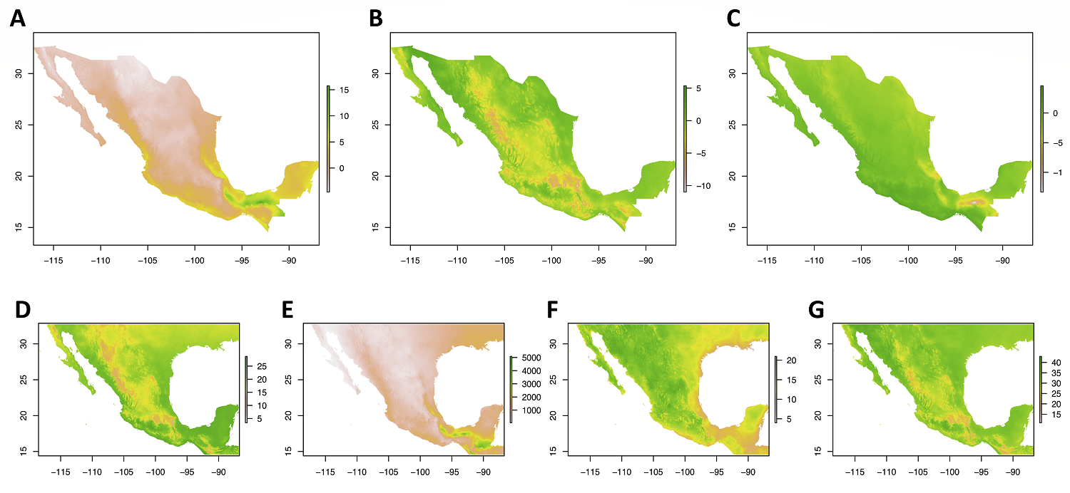
Figure 2 Climatic space in Mexico captured by the three first axes of a Principal Components Analysis of the 19 WorldClim v. 2.1 climatic variables, and four biologically important selected variables. A) PC1, B) PC2, C) PC3, D) Annual Temperature (Bio 01), E) Temperature Seasonality (Bio 04), F) Annual Precipitation (Bio 12), G) Precipitation Seasonality (Bio 15).
Realized climatic amplitude for the 139 species of Ipomoea in our final dataset across the three first climatic PCs, annual temperature and precipitation, and their seasonality are presented in Table 1. Variation in climatic amplitude is larger for PC1, followed by PC3.
Table 1 Realized climatic breadth across 139 species of Ipomoea in Mexico in the three first axes of a Principal Components Analysis of the 19 WorldClim v. 2.1 climatic variables restricted to Mexico, and four temperature and precipitation related variables. Temperature is in ºC x 10; precipitation is in mm; seasonality is calculated as standard deviation x 100 for temperature, and as the coefficient of variation for precipitation (for detailed information, see https://www.worldclim.org/data/bioclim.html). sd = standard deviation.
| Variable | min | max | mean | median | sd |
|---|---|---|---|---|---|
| Climatic amplitude on PC1 | 0.066 | 17.962 | 7.623 | 7.351 | 4.379 |
| Climatic amplitude on PC2 | 0.244 | 14.467 | 6.201 | 6.722 | 2.641 |
| Climatic amplitude on PC3 | 0.076 | 16.787 | 6.404 | 5.784 | 4.276 |
| Annual Mean Temperature (bio 01) | 0.483 | 20.717 | 10.881 | 11.958 | 4.518 |
| Temperature seasonality (bio 4) | 16 | 4113 | 1,753.832 | 1611 | 1,129.896 |
| Annual Mean Precipitation (bio 12) | 0.8 | 13.683 | 7.194 | 7.475 | 3.073 |
| Precipitation seasonality (bio 15) | 0.7 | 26.2 | 12.557 | 13.256 | 5.547 |
Climatic amplitude as a predictor of geographic range size in Ipomoea. We find that climatic amplitude accounts for a relevant portion of the variation in geographic range size across Mexican Ipomoea, from 51.5 % (PC2, on ranges calculated by buffer method) to 65.8 % (PC1, on ranges calculated by the hull method). Overall, PC1 explains the most variation on geographic range for any one method (Hull or buffer; Table 2, Figure 3). Models that include all three PCs explain 66.9 % (buffer) to 69.4 % (Hull); estimates and coefficients for models are in Table S4. Likewise, climatic breadth in temperature and precipitation related variables is also a significant predictor of geographic range, with annual precipitation breadth explaining overall a larger portion of the variance in geographic range than annual temperature breadth does (~70 % vs. 43 - 46 %, respectively; Table 2, Figure 4). Climatic amplitude related to temperature and precipitation seasonality explain intermediate amounts of variation in geographic range (44 - 54 %). For estimates and details on models see Table S4. Climatic amplitude based on annual temperature and precipitation are positively correlated (both in magnitude R 2 = 0. 0.44, and seasonality adj. R 2 = 0.368; Figure 5), so that in general, Mexican Ipomoea with small breadths in annual temperature (and its seasonality) will tend to exhibit also small breadths in annual precipitation (and its seasonality). Models that include climatic amplitude in both annual variation and seasonality explain between 60 % (temperature) and 70 % (precipitation) in geographic range variation for both Hull and Buffer calculated ranges (Table 2).
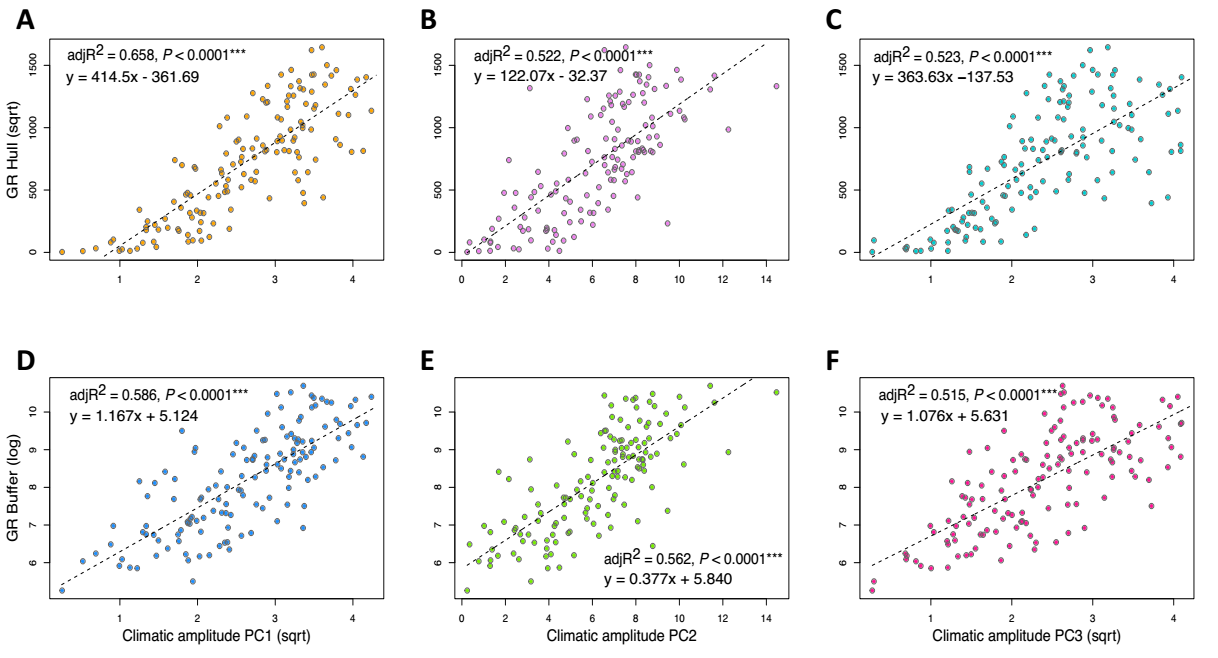
Figure 3 Climatic amplitude in each of the first three axes of a Principal Components Analysis of the 19 WorldClim v. 2.1 variables is a significant predictor of geographic range size (GR) in Mexican Ipomoea (n = 139), whether evaluated as convex Hull polygons (A-C) or buffered occurrences (D-F). PC1 (A, D); PC2 (B, E), PC3 (C, F).
Table 2 Summary of models examining climatic amplitude as a significant predictor of geographic range size across species of Ipomoea in Mexico (n = 139). Linear models were implemented using functions in base R (R Core Team 2022). For estimates and details on models, see Table S4.
| Geographic Range Hull (sqrt) | adjR2 | F-stat | DF | P value |
|---|---|---|---|---|
| ~ amplitude PC1 (sqrt) | 0.658 | 266.2 | 1, 137 | < 2.2e-16 |
| ~ amplitude PC2 | 0.522 | 151.7 | 1, 137 | < 2.2e-16 |
| ~ amplitude PC3 (sqrt) | 0.523 | 152.5 | 1, 137 | < 2.2e-16 |
| ~ amplitude PC1 (sqrt) + amplitude PC2 + amplitude PC3 (sqrt) | 0.694 | 105.5 | 3, 135 | < 2.2e-16 |
| ~ annual mean Temperature (bio 01) | 0.438 | 108.7 | 1, 137 | < 2.2e-16 |
| ~ Temperature seasonality (bio 04, sqrt) | 0.534 | 159.1 | 1, 137 | < 2.2e-16 |
| ~ annual mean Precipitation (bio 12) | 0.695 | 315.4 | 1, 137 | < 2.2e-16 |
| ~ Precipitation seasonality (bio 15) | 0.437 | 108.0 | 1, 137 | < 2.2e-16 |
| ~ annual mean Temperature + Temperature seasonality | 0.600 | 104.3 | 2, 136 | < 2.2e-16 |
| ~ annual mean Precipitation + Precipitation seasonality | 0.710 | 169.5 | 2, 136 | < 2.2e-16 |
| Geographic Range Buffer (log) | ||||
| ~ amplitude PC1 (sqrt) | 0.586 | 196.1 | 1, 137 | < 2.2e-16 |
| ~ amplitude PC2 | 0.562 | 178.4 | 1, 137 | < 2.2e-16 |
| ~ amplitude PC3 (sqrt) | 0.515 | 147.8 | 1, 137 | < 2.2e-16 |
| ~ amplitude PC1 (sqrt) + amplitude PC2 + amplitude PC3 (sqrt) | 0.669 | 94.1 | 3, 135 | < 2.2e-16 |
| ~ annual mean Temperature (bio 01) | 0.457 | 117.0 | 1, 137 | < 2.2e-16 |
| ~ Temperature seasonality (bio 04, sqrt) | 0.527 | 154.8 | 1, 137 | < 2.2e-16 |
| ~ annual mean Precipitation (bio 12) | 0.695 | 315.4 | 1, 137 | < 2.2e-16 |
| ~ Precipitation seasonality (bio 15) | 0.437 | 108.0 | 1, 137 | < 2.2e-16 |
| ~ annual mean Temperature + Temperature seasonality | 0.604 | 106.4 | 2, 136 | < 2.2e-16 |
| ~ annual mean Precipitation + Precipitation seasonality | 0.710 | 169.5 | 2, 136 | < 2.2e-16 |

Figure 4 Climatic breadth in temperature and precipitation related variables is a significant predictor of geographic range size in Mexican Ipomoea (n = 139), whether geographic ranges (GR) were calculated as convex Hull polygons (A, B, E, F), or buffered occurrence points (C, D, G, H). A, C: climatic amplitude in annual temperature (Bio 01); B, D: climatic amplitude in temperature seasonality (Bio 04, sqrt); E, G: climatic amplitude in annual precipitation (Bio 12); F, H: climatic amplitude in precipitation seasonality (Bio 15).
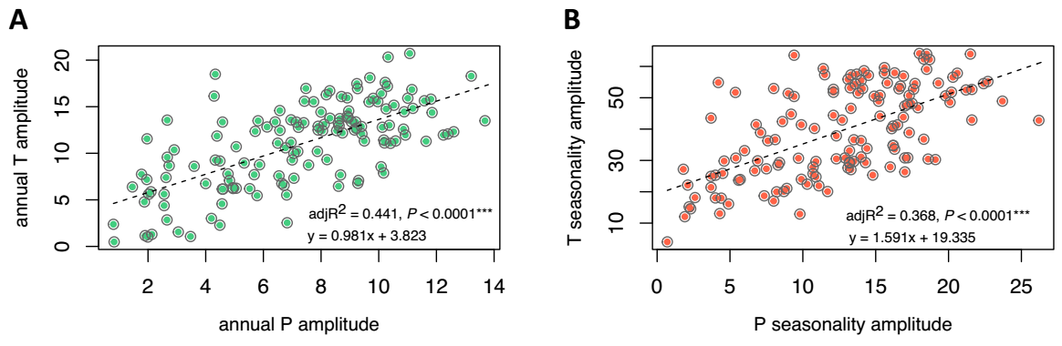
Figure 5 Climatic breadth in temperature and precipitation related variables are positively in Mexican Ipomoea (n = 139). A: annual P breadth (Bio 12) is a significant predictor of annual T breadth (Bio 01). B: breadth in P seasonality (Bio 15) is a significant predictor of breadth in T seasonality (Bio 04, sqrt).
Variability of geographic and climatic variables across the phylogeny can be visualized in Figure 6. Despite a smaller sample size (n = 59), results from our PGLS models that incorporate information on evolutionary relationships among Ipomoea species are similar to those that do not incorporate phylogenetic information (Table 3, Figure S6): a relevant portion of the variation in geographic range across Mexican Ipomoea is explained by variation in climatic breadth based on PCs (from 28.2 % for PC3, on Hull ranges to 50.2 % for PC2 on buffer ranges). This result also holds when examining climate amplitude based on annual temperature and precipitation, as well as related to seasonality in both temperature and precipitation (Figure S7). For all models, estimated lambda was zero, suggesting no phylogenetic signal in variables evaluated. Models including climatic breadth based on annual amounts and seasonality of temperature and precipitation variables explain between 44.6 % (temperature, hull method) and 67.4 % (precipitation, buffer method) of variation in geographic range. For estimates and details on all PGLS models, see Table S5.
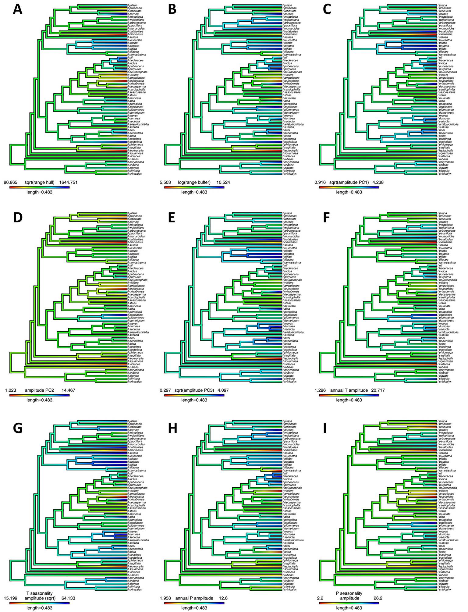
Figure 6 Visualization of geographic range size breadth and climatic amplitude in Mexican Ipomoea (n = 59) in the multigene phylogenetic hypothesis of Muñoz-Rodríguez et al. (2019). A: convex Hull polygons range size (sqrt). B: buffered occurrences range size (log) C: breadth in PC1 (sqrt), D: breadth in PC2, E: breadth in PC3 (sqrt), F: annual T breadth (Bio 01), G: T seasonality breadth (Bio 04, sqrt), H: annual P breadth (Bio 12), I: P seasonality breadth (Bio 15).
Table 3 Summary of Phylogenetic Generalized Least Squares (PGLS) models examining climatic amplitude as a significant predictor of geographic range size across species of Mexican Ipomoea in Mexico (n = 59). For estimates and details on models, see Table S5.
| Geographic Range Hull (sqrt) | adjR2 | F-stat | DF | P value |
|---|---|---|---|---|
| ~ amplitude PC1 (sqrt) | 0.474 | 53.19 | 1, 57 | < 2.2e-16 |
| ~ amplitude PC2 | 0.483 | 55.15 | 1, 57 | < 2.2e-16 |
| ~ amplitude PC3 (sqrt) | 0.282 | 23.8 | 1, 57 | < 2.2e-16 |
| ~ amplitude PC1 (sqrt) + amplitude PC2 + amplitude PC3 (sqrt) | 0.578 | 27.53 | 3, 55 | < 2.2e-16 |
| ~ annual mean Temperature (bio 01) | 0.305 | 26.45 | 1, 57 | < 2.2e-16 |
| ~ Temperature seasonality (bio 04, sqrt) | 0.372 | 35.34 | 1, 57 | < 2.2e-16 |
| ~ annual mean Precipitation (bio 12) | 0.586 | 83.23 | 1, 57 | < 2.2e-16 |
| ~ Precipitation seasonality (bio 15) | 0.364 | 34.19 | 1, 57 | < 2.2e-16 |
| ~ annual mean Temperature + Temperature seasonality | 0.446 | 24.35 | 2, 56 | < 2.2e-16 |
| ~ annual mean Precipitation + Precipitation seasonality | 0.623 | 48.95 | 2, 56 | < 2.2e-16 |
| Geographic Range Buffer (log) | ||||
| ~ amplitude PC1 (sqrt) | 0.435 | 45.64 | 1, 57 | < 2.2e-16 |
| ~ amplitude PC2 | 0.502 | 59.4 | 1, 57 | < 2.2e-16 |
| ~ amplitude PC3 (sqrt) | 0.322 | 28.58 | 1, 57 | < 2.2e-16 |
| ~ amplitude PC1 (sqrt) + amplitude PC2 + amplitude PC3 (sqrt) | 0.568 | 26.47 | 3, 55 | < 2.2e-16 |
| ~ annual mean Temperature (bio 01) | 0.402 | 39.93 | 1, 57 | < 2.2e-16 |
| ~ Temperature seasonality (bio 04, sqrt) | 0.359 | 33.53 | 1, 57 | < 2.2e-16 |
| ~ annual mean Precipitation (bio 12) | 0.553 | 72.82 | 1, 57 | < 2.2e-16 |
| ~ Precipitation seasonality (bio 15) | 0.509 | 61.19 | 1, 57 | < 2.2e-16 |
| ~ annual mean Temperature + Temperature seasonality | 0.501 | 30.15 | 2, 56 | < 2.2e-16 |
| ~ annual mean Precipitation + Precipitation seasonality | 0.674 | 60.97 | 2, 56 | < 2.2e-16 |
Species that deviate from general patterns of T and P related climatic breadth. Our approach allows identification of species that might be of interest for several reasons: species of narrower climatic breadths than expected that could be vulnerable to changing conditions; species with broader ranges than expected given their niche breadths, and species with narrow geographic ranges but broader than expected climatic breadths. Our results support that most species with narrow climatic amplitudes also have small geographic ranges, and that climatic breadth in temperature is correlated with breadth in precipitation. Yet, some species deviate from these general patterns; in this section we explore several examples of these. Ipomoea imperati, I. heptaphylla and I. violacea stand out for having larger geographic ranges than expected given their climatic breadth in temperature, precipitation, and seasonality. These species have coastal distributions (Figure S8), and this might explain that while associated with a somewhat specialized environment, they span larger geographic areas than expected. Interestingly, several species with quite narrow climatic breadths in both precipitation and temperature are distributed in proximity if not along coasts (e.g., I. gesneroides, I. lottiae, I. seannia, I. sororia; Figure 1F). Coastal environments in regard to temperature generally reflect less variable conditions than inland environments, and may buffer effects of variation in precipitation which can be more complex in relation to inland areas. The patterns we observe highlight that broadly distributed coastal species may occupy relatively narrow environmental conditions that may be changing rapidly, emphasizing issues of coastal conservation in relation to climate change.
In contrast to the species noted above, some species exhibit a relatively limited geographic distribution but have a broad amplitude in relation to some climatic variables. Examples include species occurring in mountainous areas (such as those in Baja California and Oaxaca) that might span a wide range of precipitation conditions within a relatively small geography (e.g., I. jicama and I. praecana). In addition, we note several taxa (Ipomoea chenopodifolia, I. silvicola and I. spectata) that have larger than expected temperature breadths given their rather small ranges. All three species occur in mountain ranges along the Pacific (Figure S8), where high variation in temperature can be found across small geographic areas (see Figure 2).
Discussion
We report a total of 178 species of morning-glories (Ipomoea L., Convolvulaceae) for Mexico (not including subspecific taxonomic ranks or synonyms), which is higher (by up to 19 additional species) than previous estimates (142 species reported by Austin & Huáman 1996; 159 species by Villaseñor 2016). We document a strong relationship between geographic range size and realized niche breadth (measured as current realized climatic amplitude) for Mexican Ipomoea: as much as 67 % of the variation in geographic range size across species can be explained by realized climatic amplitude. Our results are consistent with the general pattern of a positive association between geographic range size and niche breadth that has been consolidating over the last few decades across taxonomic groups and scales (Slatyer et al. 2013, Kambach et al. 2019). Incorporating phylogenetic history in our analyses (albeit in a reduced subset of our data) resulted in similar patterns, which together with all our model estimates of phylogenetic signal being zero, suggest that evolutionary history has not played a significant role shaping this pattern, and this result is also consistent with what others have found, both at regional and global scales (Kambach et al. 2019).
While a few studies have found non-positive relationships between range size and niche breadth, these report non-significant results (reviewed in Slatyer et al. 2013). One other instance found that in plants with buds near the soil surface (hemicryptophytes) range size was negatively related to germination niche (Luna & Moreno 2010) but this study differs from others, including ours, in that it addressed climatic amplitude specific to a life stage.
One of the main aspects of our work is a nuanced characterization of geographic ranges across species of Ipomoea in Mexico, one of its centers of diversity. With over 7,000 manually georeferenced records, this study contributes to closing a gap in our knowledge of geographic ranges, their variation, and putative correlates (Sheth et al. 2020) for this important group of plants, and in general. The large variability that we document in geographic range size across species (spanning several orders of magnitude) is also consistent with what others have reported, both from clade-centered perspectives, or approaches focusing on areas (Sheth et al. 2020). It has been pointed out that a sampling bias due to more widespread species being more heavily sampled and across more environments could lead to a positive relationship between range size and environmental breadth (Brown 1984, Burgman 1989). This could affect studies like ours, where range size is so widely variable. Yet, others have shown that even when accounting for sampling bias, this correlation still holds quite broadly (Slatyer et al. 2013, Sheth et al. 2020). In our case, the positive relationships we document between geographic range size and climatic breadth across an heuristic climate space (based on a 19 variable PCA) as well as climatic amplitude in annual temperature, annual precipitation, and their seasonality, held when we analyzed a reduced dataset to include phylogeny that consisted of 42 % of the original sampling. With this reduced dataset, we find the same patterns with only a small reduction in explanatory power of the models (the lowest variation explained by the reduced models was 28.2 %, compared to 43.7 % in our original models; Tables 2 and 3).
Our main approach to characterizing the climatic space available to Ipomoea in Mexico consisted of conducting a PCA on layers of 19 climatic variables, an approach that can help identify patterns of variation across multiple correlated variables. Our PCA analysis revealed that climatic patterns in Mexico are dominated by precipitation patterns (both in amount and temporality), followed by patterns of temperature variability and seasonality. Our results highlight the area of the gulf of Campeche as one where values of PC1 (which reflects precipitation and temperature seasonality) are the highest, driven by high amounts of annual precipitation (especially in the wet rainy summers) and higher winter temperatures; in this area, temperatures are towards the warmer end of the spectrum and relatively constant (with low temperature ranges and seasonality). PC2 reflects temperature (especially summer temperatures) and its constancy as well as lack of precipitation (especially in the summer), that is, how hot and dry climates are, especially in the summer. The third axis along which we characterized climate (PC3) reflects precipitation seasonality and temperature during the dry winters, as well as temperature constancy and the extent to which winters are dry.
We found that climatic breadth is a good predictor of range size in Mexican Ipomoea, both when PC axes and variables are analyzed separately or in more complex models that include more factors. So, species that have wide geographic ranges across Mexico tend to span a great deal of variability in precipitation, temperature, and seasonality, from areas where temperatures and precipitation are relatively constant (e.g., the gulf of Campeche) to areas where seasonality in these two climate components interact to yield wet but quite hot summers and drier cold winters. The variation around the general pattern of a positive relationship between climatic breadths in temperature and in precipitation that we document across Mexican Ipomoea reflects diversity in patterns of temperature and precipitation across Mexico. Plant strategies for dealing with environments that can be seasonally harsh are diverse, and many overlap with those used to face and survive in generally harsh environments (such as desert environments), including variation in life history and phenology (annual life histories, or phenological activity that includes deciduousness and dormancy during harsh conditions), as well as physiological and morpho-anatomical adaptations in leaves, stems and roots (Solbrig & Orians 1977, Lichter-Marck & Baldwin 2023). In Ipomoea, some species have annual life histories; others, while perennials, have strong phenological patterns such as dormancy during the cold dry winters, a strategy that is enabled by a combination of deciduousness and the presence of underground storage structures (Muñoz-Rodríguez et al. 2019, Wood et al. 2020). Evaluating the extent to which each of these strategies is correlated with geographic range size and climatic amplitude is beyond the scope of this study but is among the range of questions we are addressing in this group of plants in a broader context. One potential area of research is to evaluate how the positive relationship between niche breadth and geographic range size that we document varies across life history traits, anatomical adaptations, evolutionary history, and with landscape attributes (e.g., montane vs. lowland).
A potential limitation of our study is that it was circumscribed to Mexico. We decided to focus our study in an area where our confidence in manual georeferencing would be highest, but it can be (rightfully) argued that geo-political boundaries have little biological meaning. If the niche breadth - geographic range size relationship was scale dependent, we might be limiting our power to detect relationships. Not only this was not the case (as our results attest), but as others have pointed out, evidence on the limits of the niche breadth - geographic range size relationship is still inconclusive. In fact, where multiple studies have been compared, no evidence was found for differences between studies performed at local or regional scales, like ours, and those that included the entirety of species’ geographical ranges (Slatyer et al. 2013, Kambach et al. 2019). Also, of interest is to use more comprehensive or other metrics of niche breadth (Sexton et al. 2017). We focused on realized climatic amplitude as estimated from the actual points where species occur. Climatic amplitude assessed from species distribution models can be helpful in characterizing environmental distributions, especially in relation to correcting for sampling bias and for estimating the ranges of species with few known localities. Including other axes of niche breadth of known importance such as soil effects or biotic interactions (Afkhami et al. 2014, Sheth et al. 2020) would expand our understanding of the determinants of geographic range size in this important yet understudied group of plants.
Despite their limitations, studies like ours have much to contribute, not only for their potential of increasing our understanding in testing well-established hypotheses, like the niche breadth-range size hypothesis (Brown 1984, Slatyer et al. 2013), but also because their findings might have important implications for conservation. Others have elaborated on this topic, and expanded on the factors that can play a role in species range shifts as well as their contractions and expansions (Shay et al. 2021). The ‘range size vulnerability hypothesis’ (Shay et al. 2021) states that species with small geographic ranges might be at greater risk under changing climatic conditions due to their likely smaller population sizes. Thus, identifying species of potential concern is one way in which studying the relationship between niche breadth and geographic range size at local and regional scales can inform conservation decisions and even policy. In practice, this translates into locating species that deviate from a general pattern in a given clade or area. The study of factors that limit the geographic range of species that have smaller than expected ranges given their climatic amplitudes (that is, species that fall well below the regression lines in Figures 3 and 4) could be of interest from a conservation standpoint, especially if their ranges are already limited.
Also important is to identify species that despite their wide geographic ranges, have narrower climatic amplitudes than expected (that is, species that fall towards the upper left corner of the regression lines in plots of geographic range vs. niche breadth in Figures 3, 4, and S6). These species could be tracking widely available but quite specific climatic conditions, and their future could be compromised under a scenario of environmental variation. Some examples of these species are Ipomoea imperati, I. heptaphila and I. violacea (see results for details), all with coastal distributions. Another potential example could be I. pes-caprae (L.) R.Br. (Figure 1C). This species is a coastal dune specialist, with a worldwide distribution likely acquired by long-distance dispersal of seeds drifting in the ocean (Miryeganeh et al. 2014). While it is distributed around the globe, it is not found inland of coastal dunes. It is thus possible that, as sea levels rise, I. pes-caprae will face similar challenges as other species of coastal ecosystems, many of which might lose habitat to sea level rise (Nicholls & Cazenave 2010), or have their habitat replaced by other ecosystems as other species expand their ranges. For example, the replacement of salt marsh ecosystems by mangroves of the genus Avicennia (Acanthaceae) that are expanding their geographic ranges has been documented worldwide (Saintilan et al. 2014). However, different or wider niche breadths do not necessarily translate to different responses to environmental variation: in miner’s lettuce plants (Claytonia perfoliata complex), while polyploidy is associated with distinct and broader ecological niches, plants’ responses to environmental variation were similar across ploidy and niche breadth levels (McIntyre 2012, McIntyre & Strauss 2017).
Conversely, patterns in precipitation and its seasonality are important determinants of the climate in Mexico (Figure 2), as was captured by our PCA analysis (Table S2) and might shape species ranges in Ipomoea in peculiar ways. Some species that occur in the region of the Isthmus of Tehuantepec, where precipitation is abundant and seasonal, experience a narrow breadth in precipitation amount but a broad one in precipitation seasonality and temperature (e.g., I. bernoulliana, I. silvicola, I. chaenopodifilia, I. lutea). Given their breadths in precipitation seasonality, temperature seasonality, and annual temperature (but not annual precipitation, which is high in this region), these species have smaller than expected geographic range sizes. This combination of factors is consistent with a potential specialization to wet but seasonal environments that span rather narrow areas, and merits further investigation. Others have pointed out how niche breadth could narrow over evolutionary time as the result of experiencing low variation along intercorrelated niche axes (Carscadden et al. 2020).
Addressing the patterns and potential drivers of the relationship between geographic range size and niche breadth in diverse clades such as Ipomoea can contribute to our understanding of ecological amplitude (e.g., Slatyer et al. 2013, Kambach et al. 2019, Carscadden et al. 2020). It is through a more extensive investigation across ecologically and phylogenetically distant groups that patterns and their potential causes emerge. This study contributes to this question, and documents that when measured as climatic amplitude, niche breadth is a strong predictor of geographic range size in morning glories in Mexico, one of the centers of diversity of this highly diverse group of plants.
Supplementary material
Supplemental material for this article can be accessed here: https://doi.org/10.17129/botsci.3322

