


 nova página do texto(beta)
 Inglês (pdf)
 Artigo em XML
 Referências do artigo
 Enviar este artigo por email
 Citado por SciELO
  Similares em
SciELO
Similares em
SciELO 
 Permalink
Population ecology is the study of the dynamics of populations, i.e., their change in individual numbers and structure in response to abiotic and biotic factors, and of the ecological and evolutionary consequences of these changes. A glance at current textbooks reveals the diversity of topics studied by population ecology, from the essential study of the causes and consequences of population growth to interactions between species, life history evolution, the determinants of community structure, and the management of populations and communities for biodiversity conservation (Ranta et al. 2005, Begon et al. 2009, Vandermeer & Goldberg 2013).
In population ecology, demographic models constitute a conceptual and practical tool fundamental for the elucidation of the causes and consequences of population dynamics. The information derived from these models has direct application in species conservation and management, as well as in determining how their life histories evolve in response to environmental factors and species interactions. The different forms of expressing population growth rate (as lifetime contribution to reproduction R, the ratio in the number of individuals over two consecutive time intervals λ, or a compound rate over time r) are used not only as descriptors of the current dynamics but are key to determining, for example, levels of protection or harvest to keep the population stable or as fitness measures useful in an evolutionary context.
In this paper we specifically concentrate on structured population models, which incorporate the change in individual demographic processes (fecundity, ontogenetic development -often referred to simply as growth- and survival, also called vital rates) in the course of the life cycle. Over the last half century, population ecologists have employed these models to record the dynamics of a wide variety of wild, threatened, invasive or economically important species (Crone et al. 2011, Doak et al. 2021). The growth in the number of studies is witnessed by the COMPADRE database which currently contains 8,708 matrix population models of 757 plant species from 639 publications (COMPADRE 2021). Thanks to this volume of information, broad patterns of demographic variation in plants have been identified. For example, we know that many natural populations are close to stable population size and structure, and that the persistence of long-lived species is owed more to the survival of adults than to the recruitment of seedlings, while the opposite is true of short-lived herbs (Silvertown et al. 1993, Franco & Silvertown 2004). Consequently, demographic processes correlate more with functional attributes of the species (Poorter et al. 2008, Adler et al. 2014) than with their geographic or phylogenetic proximity (Coutts et al. 2016). Elucidation of such broad patterns may give the impression that it is no longer necessary to conduct studies of individual species whose demography can be readily characterised by reference to their life history. This may be true if the objective is simply to confirm these patterns, but since no two species or populations and the conditions under which they are found are alike, such an approach may provide general rules of thumb but not be a reliable practice if the objective is to provide specific conservation and management actions under particular conditions. This is clearly the case in risk assessment of both threatened and invasive species.
The world is changing rapidly, and demography is advancing towards an understanding of populations as they and their environment are transformed. In a stable world, factors such as the environmental conditions and population density remain relatively constant, and (unless the research question requires it) they need not be considered explicitly in the demographic models any more than other variables assumed constant. However, for many applications the correct representation of populations in a changing world requires the consideration of the context in which the populations develop (Crone et al. 2013, Ehrlén et al. 2016). This is particularly important for plants because, ignoring the issue of resource distribution, they cannot move to areas where the physical environment is appropriate with sufficient speed to keep pace with it (Crone et al. 2013). The consideration of the dynamics of populations away from equilibrium thus becomes a subject of growing interest.
In this contribution we revise prominent conceptual and methodological issues in structured projection models as they apply to plant populations. In the first section, we revise the basics of projection models in order to set the basis for the following sections; a more detailed discussion of these models can be consulted elsewhere (Caswell 2001, Ranta et al. 2005, Gotelli 2008, Vandermeer & Goldberg 2013, Merow et al. 2014a, Rees et al. 2014, Ellner et al. 2016). In the second section, we discuss the construction of projection models in plants, including the selection of the state variable, model parameterisation, and some commonly encountered problems in model construction. In the next section we discuss populations in their context: temporal changes -with emphasis on transient dynamics-, conspecific density, environmental factors, and space (Figure 1). Based on these ideas, we conclude with some general considerations on how to choose a suitable model and handle the variables in it.
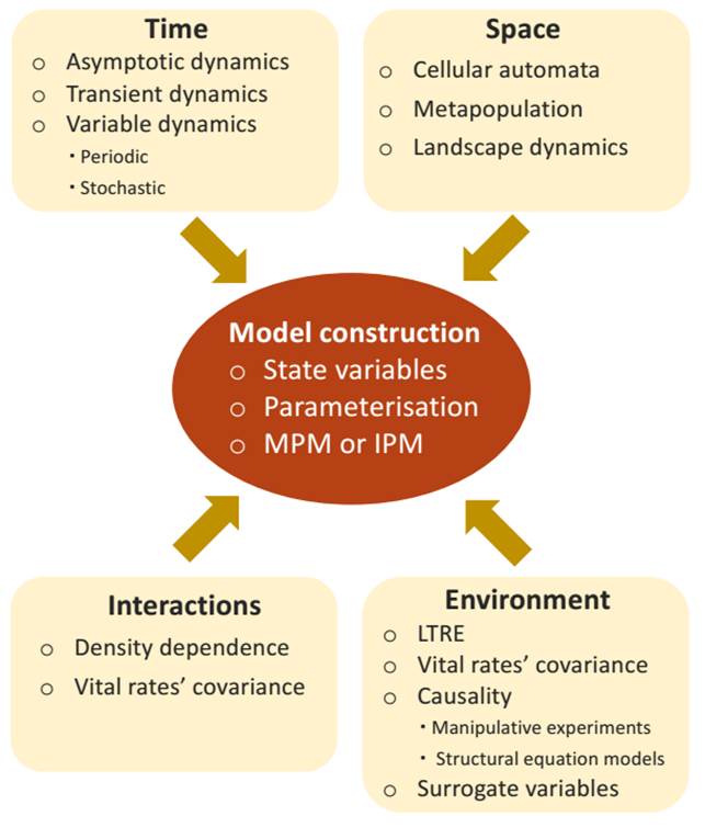
Figure 1 The essential elements for the construction of a structured population model depending on the factors that are considered explicitly in it, the physical dimensions in which the population develops, and the environmental and biological influences that affect it.
Structured projection models: their logic, construction, and basic analysis
The growth of populations lacking structure. In order to review the conceptual and methodological assumptions made in the analysis of population dynamics, we need to start with the simplest model on which all others are built. This model assumes a closed population (one with no migration) where no differentiation of individuals (by sex, age, size, or any other state variable) is taken into account. It is also assumed that the behaviour of the population at any time is independent of its history, and only depends on its current condition. In this simple scenario, the rate of change in the number of individuals (N) from the beginning to the end of a time interval (t to t + 1) is determined by the population capacity for growth given by the difference between births and deaths and summarised in one parameter, the finite rate of population increase (λ):
With the additional assumption that λ is constant, projection over a number of time intervals, say between time zero and time t, leads to the general equation
The assumption of constancy in λ implies resources are not limiting for the timespan under consideration (t) and that environmental conditions remain unchanged. Under real circumstances, this assumption can only hold for very short timespans.
Structured population models. Equations (1) and (2) may be useful in cases where a simple count of the number of individuals is all that is required, but when information on the age and/or size of individuals is relevant, the model leaves this essential information out. For example, in the case of modular organisms such as plants, one million tree seedlings may not even come close to the biomass, and hence energy budget, effect on neighbours and effect on other species sharing the same habitat, of a single adult tree. Structured population models acknowledge that individuals differ in their demographic properties as they age, grow and move through the different stages of the life cycle, and that these differences determine their contribution to population growth (Caswell et al. 1997). The dynamics of structured populations at a given time also depends on the population structure, which is the composition of the population in terms of the abundance of individuals in different stages of the life cycle (de Roos 2020). The growth of the population in the short term will not be the same if it is composed mostly of seedlings or only of reproductive adults.
A fundamental element of structured models is therefore the state variable, the variable that best correlates with the changing demographic properties of individuals as they progress through the life cycle. The state variables most often considered to structure plant populations are age, developmental stage, and individual size (Caswell 2001). Sometimes two or more state variables are considered in the model (e.g.,Law 1983, van Groenendael & Slim 1988). The state variable can be discrete or continuous. Matrix population models (MPMs) organise individuals into subsets along the life cycle, such as seeds, seedlings, juveniles and adults, their corresponding ages or sizes. If other types of propagules exist, such as bulbils or clonal recruits, these can be incorporated in additional stages. When the state variable is explicitly modelled as continuous (or a combination of discrete and continuous), an equivalent integral projection model (IPM) may be used.
In matrix models, instead of a scalar N t defining population size at a given time, the population is represented by a vector of abundances for each stage (say, stages 1 to m) at a particular time (t):
To estimate the change in each element from one time to the next, a series of linear functions is required (Leslie 1945, Lefkovitch 1965, Caswell 2001):
This system can be written in matrix form as:
It can also be written in condensed form as:
As with the unstructured population model, equation 4 can be projected over a time interval from zero to t yielding:
The square matrix A contains all the linear coefficients [a ij ] describing the possible transition and/or contribution of an average individual in stage j at time t to stage i over the time interval t to t + 1. Matrix coefficients are the product of two or more vital rates (Caswell 2001, Franco & Silvertown 2004, Kendall et al. 2019). For example, for individuals that transit to a category of larger-sized plants the matrix coefficient is the product of two vital rates: the probability of surviving over the time interval and the probability of growing into the specified larger category. Some matrix coefficients may represent transitions that were either not observed or do not exist at all, such as individuals growing across several size classes in a unit time interval. This depends on the stage classification employed, which ought to be chosen judiciously based on both biological and statistical grounds (Vandermeer 1978, Moloney 1986, Enright et al. 1995).
The similarity between equations 1 and 4 (and between 2 and 5) is more than superficial. Implicit in matrix A is its mathematical solution yielding a parameter value both conceptually and methodologically equivalent to λ, hence represented also by this Greek letter. This is the largest of the m possible solutions or eigenvalues of matrix A , and thus is known as the dominant eigenvalue (Leslie 1945, Caswell 2001). The other eigenvalues determine other aspects of the population’s dynamics (see section Temporal variability). Associated to λ, there are two vectors, represented by w and v and called the dominant right and left eigenvectors, that correspond to the stable population structure (stable stage distribution or SSD, the expected proportion of individuals in each stage) and the distribution of reproductive values (the proportion of expected future offspring at each stage), respectively (Leslie 1945, 1948, Caswell 2001). The parameters λ, w and v are often used as standards to be compared across sampled populations or species. They are referred to as asymptotic properties of the model because the methods employed to estimate them converge on their values asymptotically. In the power method, equation (4) is iterated (i.e., it is repeatedly applied to project the population over time, one step at a time) and the modelled population approaches a constant growth rate, a stable structure, and stable reproductive values. An unfortunate consequence of the latter method is that it insinuates the model is being extrapolated into the future, thus implying unlimited population growth, which is obviously impossible in a world with finite resources. However, as an analytical property of the characteristic equation, λ measures the rate of population increase when the population structure corresponds to that in w . As such, it does not involve any projection over time; despite this, the notion that the eigenvectors and eigenvalues involve necessarily a future state persists and it has not been solved by the use of the terms projection and forecasting (i.e., prediction) to differentiate between the two interpretations: (i) the model as a statement of properties (λ, w and v) for the population at the time it was observed (implied by the analytical methods), or (ii) as indices of how the population might behave for at least some time into the future (evoked by the iterative method). The second interpretation should always be made with care in growing populations. It is more easily justified in the case of declining populations because in this case resources are generally not an issue (Morris & Doak 2002, Juárez et al. 2014).
In the case of an IPM model, its core is made of vital rate functions: s(z), describing survival probability over the state variable z; g(z', z), the probability that an individual in state z at time t transits to state z' at time t+ 1 given that it survives; and f(z', z), the number and size of offspring (z’) produced by an individual as it progresses through the state variable (z). The three functions are integrated into a kernel K. The essential structure of the kernel is:
More complicated structures with more functions can be employed if necessary to represent more complex life cycles, e.g., using different functions to include sexual reproduction and vegetative propagation instead of a single fecundity function. The kernel function is thus conceptually equivalent to the transition matrix A and the population is projected over time using the discrete-time model:
where n t (z) is a function that describes the number of individuals in state z at time t, and is equivalent to n t in equation 4; Ω stands for the range of the state variable; and the integral combines the product of the kernel and population abundance over the entire range of the state variable. In order to construct the kernel, one has to choose the form of the individual functions for survival, growth and fecundity employing standard regression methods. If the state of individuals includes both discrete and continuous variables (for instance, germination introduces a sharp divide in the life cycle, and the fate of seedlings may depend on their initial size), two categories will be needed to distinguish between seeds and newly established plants, which are subsequently described using a continuous function of size. General IPMs have been developed to deal with these cases. These models also allow the simultaneous use of more than one state variable (Ellner & Rees 2006).
The advent of the more versatile IPMs does not mean that MPMs must be abandoned. Doak et al. (2021) compared key outputs from both approaches (population growth rate, sensitivity and elasticity patterns, life expectancy and damping ratio; some of these parameters are defined later) and found no large differences between models, especially when MPMs were built using ten or more categories. Arguments in favour of MPMs are ease of construction and interpretation. MPMs also avoid the need to choose from a range of possible mathematical functions (as in IPMs) when there is no clear indication why a particular function ought to be preferred apart from statistical expediency. This said, it has also been suggested that IPMs could benefit from the use of spline functions that preserve the empirically observed shape without committing the user to simple functions with little biological justification (Dahlgren et al. 2011). IPMs avoid the often-arbitrary discretisation of what may be a clearly continuous state variable, such as age or size. In terms of output, λ values are broadly independent of the categorisation used in MPMs and similar to those obtained from IPMs (Easterling et al. 2000, Ramula & Lehtilä 2005, Ramula et al. 2009, Salguero-Gómez & Plotkin 2010, Dahlgren et al. 2011, Doak et al. 2021). Biased λ estimates may nevertheless be obtained when using too few categories. IPMs can accommodate covariates, such as density or environmental factors, and covariances between demographic processes with greater ease and versatility than MPMs (Ellner & Rees 2006, Doak et al. 2021, Ellner et al. 2022).
Sensitivity and elasticity in plant populations. An important question in the analysis of structured population models is the quantification of either the absolute or the relative effect that a change in a particular element of the matrix or the kernel has on the attributes of the population, such as the population growth rate. This effect is known as sensitivity. This can be calculated by numerically changing the matrix coefficients or the kernel parameters, one at a time while holding all others constant, and observing the effect on the parameter of interest, such as λ or population size (Caswell 2001, Griffith 2017). In MPMs, a preferable alternative to changing the values of the matrix coefficients is to consider the vital rates embedded in them (Caswell 2001). The estimation of the sensitivity of λ to changes in a matrix coefficient is so widespread that the term sensitivity on its own has become a synonym of this scenario. However, as Caswell (2001) points out, a precise description of what parameter is being altered and what population attribute the consequences are being measured on must be provided. The sensitivity s ij of λ to changes in a coefficient a ij can be estimated as the slope of the relationship between both parameters:
This sensitivity can be calculated from the two dominant eigenvectors v and w (Caswell 1978).
Sensitivity measures an absolute effect. However, given that vital rates are measured on different scales (e.g., survival can only have values between zero and one while fecundity does not have a mathematical maximum value -though it obviously has a finite, biologically possible maximum), it is often convenient to estimate the effect that a proportional change in a matrix element or vital rate would have on the corresponding proportional change of λ. This is known as elasticity and its definition when investigating the effect of changes in matrix coefficients on λ is (de Kroon et al. 1986, Caswell 2001):
Elasticity plays an important role in comparative demography, the study of the variability in population dynamics across species and the factors that shape that variability. Elasticities in structured population models can be used to produce a type of ordination using the elasticity of the three basic demographic processes and offering a convenient way to compare species or populations. Because elasticities are measured on a relative scale, i.e., together they add up to one, the total elasticity for each of these three processes can be plotted in a ternary graph or “demographic triangle” (Franco & Silvertown 2004). Originally, it was proposed to employ the elasticity of matrix coefficients assuming that their position in the matrix approximately reflected one of the three demographic processes of survival, growth, and fecundity (Silvertown et al. 1993). However, matrix coefficients are combinations of the basic vital rates —equations 1-5 in Franco & Silvertown (2004)— and it is the elasticity of the latter that should be employed when positioning populations in the demographic triangle —equations 7-11 in Franco & Silvertown (2004) —. If the sampled population(s) of a species accurately represents the typical demography of a species, plotting the elasticity value of the three components on λ in the demographic triangle defines the position of the species in elasticity space. The position of species in elasticity space correlates with both life history parameters (e.g., lifespan and generation time) and indices of population dynamics (e.g., intrinsic rate of population increase and damping ratio; Franco & Silvertown 2004). Despite the more expedient way to estimate the elasticity of matrix coefficients than that of vital rates, it must be emphasised that the elasticity of the underlying vital rates is the only unambiguously interpretable calculation. The use of elasticity of matrix coefficients on λ as axes of the demographic triangle should therefore be discouraged.
Uses of projection models in plant ecology.Crone et al. (2011), in a review of the application of MPMs by plant ecologists over the past 50 years, found that these models have been used mostly to derive basic information on species or with the intention of using the results for management or conservation purposes. Most studies were limited to the calculation of λ and of sensitivities or elasticities. The literature was dominated by short term studies (< 3 y) conducted in one or a few sites, so temporal and spatial variability had not been assessed in detail. Doak et al. (2021) found similar patterns after analysing the articles published between 2002 and 2018. Despite the relatively narrow scope of the majority of the demographic studies, the range of topics that have motivated ecologists to use projection models is noteworthy. Up to the first decade of this century, few studies had analysed how vital rates and populations responded to conspecific density, fire, climate change or floods (Crone et al. 2011). However, this has begun to change rapidly over the last decade (Ehrlén et al. 2016). Projection models have also been used to analyse population viability, the dynamics of biological invasions, the costs of reproduction, eco-evolutionary dynamics, multispecies interactions, spatial structure of populations, demographic and environmental stochasticity, habitat fragmentation, and life-history evolution (see Caswell 2001, Crone et al. 2011, Ellner et al. 2016 and references therein), among many others.
Given the wide use of projection models for species management and conservation, their capacity to forecast the population growth rate or size in the future becomes important. However, as pointed out by Caswell (1989), projection models do not pretend to predict the population’s future. Moreover, Crone et al. (2013) found that projections of MPMs poorly matched the changes in population size observed a few years later, concluding that projection models should not be used to forecast population status.
The challenge of building a robust projection model
The wide spectrum of applications and the availability of software that facilitate the analysis of projection models have contributed to their acceptance and widespread use. In order to make the most of their widespread use, however, it is worth becoming familiar with some common mistakes. These include problems of matrix parameterisation, such as inclusion of a seed category that artificially delays seedling recruitment by one year when (some or all) seeds produced at time t germinate and produce recruits by the next census, t+ 1 (Caswell 2001), and survival values of adults and/or recruits inadvertently ommited from the calculation of a coefficient (Kendall et al. 2019).
On the practical fieldwork aspect, the lack of knowledge on certain stages of the life cycle (e.g., whether the species forms a seed bank, propagates vegetatively underground or some individuals go dormant for a variable number of years) makes it difficult to incorporate these aspects in the model. In other cases, limitations of fieldwork preclude the collection of information on important demographic processes, such as the episodic recruitment or death in long-lived species (e.g., the Saguaro, Carnegiea gigantea; Félix‐Burruel et al. 2019). There are excellent texts on how to build MPMs (Caswell 1997, 2001, 2019) and IPMs (Merow et al. 2014a, Rees et al. 2014, Ellner et al. 2016) correctly, so we will focus on two aspects that, in our experience, are frequently debated in plant population ecology: the selection of the appropriate state variable and the parameterisation of the model.
State variables. There has been some discussion in the literature as to which state variable is best at describing and quantifying the three essential demographic processes in plants. In particular, the discussion has centered on whether these three attributes better correlate with age or size, which should routinely be tested (altogether with different formulations of “size” such as height, volume or number of modules) when constructing any particular model. While the choice between age and size is evidently a matter of empirical evidence, it is also a red herring: the life cycle occurs over a temporal scale, and although its duration varies from individual to individual, time is implicit in the vital rate growth. It is therefore possible to reconstruct an age-based life table, as well as to quantify variability in size by age, and variability in age by size, from an MPM (Cochran & Ellner 1992), and similarly from an IPM. Given the variety of life histories (i.e., the timing and manifestation of attributes of the life cycle), whether a sufficiently detailed model can be constructed is a matter of sample size, and thus manpower. Nested MPMs that include both age and size have been produced (Law 1983, van Groenendael & Slim 1988), but the amount of information required to nest state variables increases exponentially with both the number of variables and the number of categories within them. Equivalent models have been used for IPMs, involving the regression of the vital rates on age and size during model fitting (Childs et al. 2003).
Model parameterisation. When building a model, the legitimate question of which is better, an MPM or an IPM is likely to arise. There has been some recent debate on this topic (Doak et al. 2021, Ellner et al. 2022) but much of the contention is a misunderstanding: both alternatives are in fact conceptually equivalent and none is intrinsically better in every scenario. Thus, we will only delve into the differences between MPMs and IPMs when the distinction is relevant for a certain application. Given that the analysis of IPMs involves the discretisation of the kernel, effectively turning it into an MPM with many categories (Ellner et al. 2016), the only difference between both approaches in practice is the way in which the matrix is parameterised.
MPM parameterisation is straightforward: the probability that an individual in category j reaches category i at time t+ 1 is calculated using a frequentist approach, e.g., it is calculated as the fraction of survivors in category j that were observed to transit to category i. In contrast, transition probabilities and individual fecundity in the discretised IPMs are not calculated from raw counts but from regression models fitted for each vital rate (Ellner et al. 2016). In both cases, data usually come from tagged plants that are followed over time periodically (usually annually for perennial plants) recording their survival, growth and fecundity (Caswell 2001).
Estimating vital rates from follow-up data is typically a simple task. However, some rates may be difficult to estimate in plants and potentially have a significant effect on model output. Such rates generally occur at both ends of the life cycle, i.e., during recruitment and death. In IPMs, uncertainty about the fitted functions increases at both extremes of the state variable, aggravating this problem (Merow et al. 2014a). Seeds are not easy to count on the mother plant, their dispersal is difficult to monitor, and they may become buried for many years before germinating. Inaccurate fecundity estimates arising from such difficulties are likely to have a larger effect on λ in short-lived herbs or growing populations with high elasticity of recruitment (Silvertown et al. 1993, de Kroon et al. 2000). Fecundity can be obtained through the mechanistic approach (Menges 1990) from values for each step in the events linking the adult to the seedling. Such chains can be quite long, e.g., number of germinants = fruits produced × number of seeds per fruit × fraction of viable seeds × fraction that escapes predation × probability of reaching a safe site (sensuHarper et al. 1961) ( probability of germinating. Many of these figures are difficult to estimate realistically. In the empirical approach, recruitment is estimated from simple calculations based on some measure of reproductive output per individual in each stage (j), times a conversion factor that turns such output into the observed number of recruits, usually via the “anonymous reproduction” method (Menges 1990, Caswell 2001).
At the other end of the life cycle, mortality of large adults is a rare event in long-lived perennials, and it is not easily observed unless a very large sample is available. This leads to overestimation of survival and λ, as well as of other life history parameters. To solve this problem, Silvertown et al. (2001) artificially decreased the value of survival in the last stage for Avicennia marina and Astrocaryum mexicanum reported by Burns & Ogden (1985) and Piñero et al. (1984)), respectively, to a value that matched their maximum longevity estimated by the authors from growth data. This correction was feasible for plants whose maximum size and the relationship between size and age were known (usually trees) but may be more difficult to ascertain in other life forms. In IPMs, the use of the logistic function (which has an upper asymptote at a value of one) to model survival frequently results in immortal large plants (Merow et al. 2014a), in which case an alternative function should be used (e.g.,González & Martorell 2013).
Other methods have been developed over the last decade to deal with data that, from a practical point of view, cannot easily be obtained from the monitoring of individuals because they are too rare or would have to be observed over decades, if not centuries. Both interpolation and extrapolation can also be used in either MPMs or IPMs to estimate missing vital rates (Ramula et al. 2009, Peters et al. 2011, Tremblay et al. 2021). Alternatively, inverse estimation of vital rates can be achieved from information on population structure and size. This process has been used to calculate missing components of the life cycle, complete projection models, or long-term changes in population dynamics such as those expected during succession or under the influence of climate change (Ghosh et al. 2012, Martorell et al. 2012, González & Martorell 2013, González et al. 2016).
These problems highlight the issue of the size of the data set, which has a far larger impact on the accuracy of the results than the modelling approach (Doak et al. 2021). It has been proposed that IPMs are more efficient than MPMs when dealing with small datasets (Ramula et al. 2009, Ellner et al. 2022) but Doak et al. (2021) did not find conclusive evidence on this issue. Sampling protocol is important here: if efforts are made to sample equally all categories, the type of model is not overly relevant. However, under random sampling or when efforts to sample underrepresented categories fail, small samples result in inaccurate or missing matrix coefficients, and IPMs perform better (Ellner et al. 2022).
An important issue when building IPMs is defining the form of vital rate functions. This relationship is likely to be nonlinear, and, as in most dynamical systems, the specific form of the non-linearity is critical (see Martorell 2014 and references therein). The use of alternative functions to model a vital rate has been shown to have a sizeable impact on the projected behaviour of the population (Dahlgren et al. 2011, González et al. 2013), indicating that a poor function choice will lead to erroneous estimation of model outputs. Different functions may fit the data equally well yet having very different biological interpretations. As we will see, this problem, known as structural uncertainty (Eager et al. 2012), will appear repeatedly when building projection models. A partial solution to this problem when using IPMs is to “let the data speak for themselves” by fitting a smooth function that follows the data closely with no a priori function selection by the researcher, using, for example, generalised additive models (Dahlgren et al. 2011, González et al. 2013, Rees et al. 2014). However, such methods require large datasets and may depend heavily on which statistical procedure is used. Methods that favour the match between data and function may lead to overfitting and overly wiggly relationships (e.g., restricted cubic splines; Dahlgren et al. 2011, Harrell Jr 2017). Methods that penalise relationships with many parameters reduce the problem of overfitting but tend to produce linear functions where additional information would suggest otherwise (e.g., penalised thin-plate splines; Wood 2017, Merinero et al. 2020) Another aspect of structural uncertainty arises when dealing with the functions that determine growth (g(z',z)). In this case, the distribution of the model is likely to have a large impact on the projected population dynamics because it determines the state of individuals in the future and thus other vital rate values in the successive iterations of the model. In addition, symmetric distributions commonly used in regression analysis, such as the Gaussian, are unlikely to represent the data appropriately. For instance, when measures of stem circumference are used as state variable, reductions in size are unlikely and growth would nearly always be positive, while the opposite may occur when using variables that may undergo dieback or herbivory (DeMarche et al. 2019, Doak et al. 2021). MPMs, on the other hand, do not rely on a priori functions and distributions, and in this sense are “agnostic about… vital rate patterns” (Doak et al. 2021).
Demography in an environmental context
Temporal variability: stochastic and transient dynamics. Despite the natural tendency for structured populations to tend towards asymptotically stable parameter values (a property known as ergodicity), it is evident that population numbers, growth and structure vary both spatially and temporally in natural populations. The causes for this variation are many and, ignoring the specific effects of biological interactions, are covered under the subject of demographic and environmental stochasticity, which also incorporates periodic variability (Caswell 2001). Although we cannot do justice to these types of models here (there are excellent texts on the subject; Caswell 2001, Tuljapurkar 2013), it is pertinent to highlight that they share some of the ergodic properties of the standard model, with the caveat that, unlike the latter, the ergodic properties of stochastic and periodic models apply to their mean values (such as their mean λ and the average proportion of individuals in each stage of the life cycle).
While the asymptotic ergodic properties of deterministic, stochastic and periodic models make them important tools for population projection, the subject of the consequences that disturbance to the structure of a population has on its short-term dynamics (transient dynamics) is of great practical interest, particularly in conservation biology (Koons et al. 2007, Stott et al. 2011). For example, plant colonisation of a new habitat generally occurs via propagule dispersal. These propagules will take some time to develop and eventually reproduce. Thus, the dynamics of colonising populations starts far from SSD, and our understanding of the colonisation process may benefit from an analysis of the population trajectory under these rather different initial conditions (Jelbert et al. 2019). The same is true for studies on biological invasions, population recovery after a disturbance such as hurricanes, wildfires or harvesting events, or if the population is heading to a new equilibrium. Transient dynamics can be investigated directly by projecting the changes in population structure given an initial population and the measured vital rates summarised in a transition matrix. This simple method provides a direct answer to the question of how the population structure is likely to vary in the immediate future if the estimated vital rates are indeed similar under colonising conditions (e.g.,Caswell & Werner 1978). There is no guarantee, however, that the vital rates will have the same values when population size and structure are drastically different. Despite this possibility, assuming that the model fairly represents a typical cohort for the subject population provides the opportunity to investigate its likely transitory behaviour.
Traditionally, two analytical indices based on the mathematical properties of the observed model have been estimated: the damping ratio and the period of oscillation. The damping ratio is the ratio between the dominant eigenvalue of the matrix and the absolute value of the second largest eigenvalue (formula 4.90 in Caswell 2001). This dimensionless ratio is larger as the difference between these two eigenvalues increases, meaning that the dynamics is mostly determined by the dominant eigenvalue and the population converges rapidly on SSD. Obviously, if their values are closer, convergence towards SSD will be slower. The period of oscillation, on the other hand, measures the number of time units (usually years in models of perennial plant populations) that an oscillation lasts. It is calculated as the angle between the dominant eigenvalue and the largest complex eigenvalue in the complex plane (Formula 4.99 in Caswell 2001). Typically, populations do not converge towards their asymptotic state monotonically, but show oscillations due to the contribution of all eigenvalues -in simple terms, a consequence of the changing proportions of non-reproductive and reproductive individuals. The overall dynamics is dominated by the larger eigenvalues, thus the use of the two larger eigenvalues (real or complex) in these two indices.
Indices that measure differences between observed and stable population structure have been proposed. Three such indices are: (i) Keyfitz’s Delta (the distance between two probability vectors, i.e., that between observed and stable stage distributions scaled as proportions; e.g.,Keyfitz 1968, Williams et al. 2011, Jäkäläniemi et al. 2013), (ii) Cohen’s cumulative distance (their cumulative distance between an observed or hypothesised vector and the projected SSD considering the population’s trajectory over time; Cohen 1979, Williams et al. 2011), and (iii) projection distance (the proportion of an observed vector that parallels SSD taking into account both the differences between observed and expected proportions and the reproductive value of each stage; Haridas & Tuljapurkar 2007, Williams et al. 2011). In addition, several indices of the oscillatory behaviour of populations as they tend towards SSD have also been proposed. These indices can be classified into those that measure the change in population size over one time-step, those that quantify the maximal possible difference in population size, and those that are related to asymptotic population size; some include measures of both attenuated and amplified dynamics (lower and higher density than expected, respectively; Stott et al. 2011). Examples of their application are many and will not be described in detail here (e.g.,Townley et al. 2007, Townley & Hodgson 2008, Ezard et al. 2010, Stott et al. 2010, 2011, 2012, Williams et al. 2011, Ellis 2013, Tremblay et al. 2015, Iles et al. 2016, McDonald et al. 2016). However, the different transient indices are correlated with each other (Table 2 in Stott et al. 2010), as do the damping ratio and the period of oscillation (Table 1 in Franco & Silvertown 2004), indicating that they are largely redundant (Stott et al. 2010). Damping ratio and oscillation period also show strong relationships with other life history attributes, such as lifespan (negative and positive, respectively; Franco and Silvertown 2004).
Density-dependence. Despite their tendency to grow indefinitely, population sizes remain relatively stable (Roughgarden 1979, Begon et al. 2006). This is a likely result of the effect of population density on vital rates, which has been known for a long time (Harper 1977). The role of density-independent factors, such as disturbances or climatic variability in determining population size has been acknowledged since the mid 20th century (Andrewartha & Birch 1954). Hurricanes, fires or droughts may cause severe reductions in plant numbers. The ensuing recovery of populations can be analysed using the methods discussed in the previous section. In many cases, such events occur randomly or cyclically over time, and thus stochastic or periodic projection models are an appropriate choice to study the effects of density independent factors. Nevertheless, in the long run, populations whose dynamics are determined solely by environmental fluctuations are still expected to grow or shrink exponentially (Tuljapurkar 2013) because they lack the feedback provided by density dependent factors. Density-dependent regulation allows populations to persist, because they can grow when small, while setting a limit to their size as they become large.
A variety of widespread processes, such as intraspecific competition, abundance of specialist predators or soil microorganisms correlate with population density (Case 2000, Chesson 2000, Bever 2003). The mechanisms behind density-dependence should ideally be considered in projection models because they may affect the dynamics of populations differently (Case 2000, Tilman 2007, Topping et al. 2015). However, determining which factors regulate population size requires observational and experimental studies that are not frequently conducted.
The indeterminate growth of plants, which potentially leads to increases in size of several orders of magnitude, particularly in trees, requires consideration of their size in the quantification of density. It also means that interactions between individual plants depend strongly on their sizes. For instance, seeds compete with other seeds for safe sites where successful establishment may occur (e.g., Childs et al. 2004, Noël et al. 2010), and tall plants affect smaller ones more than they affect similarly sized or taller plants when competing for light. In consequence, asymmetry is the rule in plant-plant interactions (Weiner 1990).
Density dependence is frequently incorporated in projection models by expressing vital rates not as constants but as functions of density with two important considerations (Caswell 2001, Ellner & Rees 2006). Firstly, vital rates are not functions of the total number of individuals but of a subset of the population, and different individuals can be weighted depending on the magnitude of their effect (Ellner & Rees 2006). Secondly, the effect of density depends on the status of the individuals that are affected. In IPMs, changing effects of density dependence over the whole life cycle can be incorporated via multiple regression by including the effect of density and its interaction with the state variable in the vital rate functions (Dahlgren et al. 2014). The equivalent scenario in MRMs means that either each matrix coefficient would have its own response to density (e.g., Stokes et al. 2004, Pathikonda et al. 2009) or a common response if regression methods of the response across stages is employed (Feldman & Morris 2011). Alternatively, the projection of density-independent models for different populations at a range of densities treated as a discrete factor have often been compared directly (Piñero et al. 1984, Meekins & McCarthy 2002, Gustafsson & Ehrlén 2003, Fréville & Silvertown 2005, Gornish 2014). This has the advantage of not requiring the specification of any function, avoiding the problem of structural uncertainty. For further details consult section Abiotic environment below, where we discuss the incorporation of environmental factors to projection models; many of the considerations there are valid for the inclusion of density dependence as well.
Due to the expectation that density-dependent regulation is pervasive, some ecologists have called for its routine inclusion in demographic studies to increase their predictive power (e.g., Bierzychudek 1999, Ramula & Buckley 2010). However, the capacity of density-independent models to forecast population sizes in nature is independent of the strength of density dependence (Crone et al. 2013), suggesting that the incorporation of density dependence does not affect model realism. If the population density is stable, its effect is already implicit in the observed vital rate values and, therefore, incorporating it explicitly in the model would not represent an improvement. Another possible explanation for the sufficiency of density-independent models is that there are several complications in detecting and modelling density dependence, which are frequently overlooked. Ignoring them may result in muddled or spurious density effects that do not improve model performance. Among these complications are:
Spatial scale.- Density dependence is usually measured using data from plots with different densities. However, the interactions that underlie density dependence often occur over very small spatial scales, such as the competition between a plant and its immediate neighbours. Consequently, the use of an overall plot-wide measure of density is likely to miss its more immediate neighbour effect on individuals. The use of small plots, on the contrary, increases noise in the data due to inherent effects of small sample size and demographic stochasticity (Freckleton & Watkinson 2001), making density-dependence harder to detect and describe correctly.
Structural uncertainty.- Characterisation of density dependence involves the selection of a function that correctly describes the relationship between individual performance and density. Such relationship is usually non-linear, and using different functions can have large impacts on model projections (Eager et al. 2012). As it happens when modelling vital rates themselves, the selection of different functions is guided more by statistical expediency than by an understanding of the mechanisms responsible for the shape of the functions chosen. Having said this, density dependence in plants usually takes the form of a hyperbolic or Beverton-Holt function (Freckleton & Watkinson 1999). This function does not produce overcompensation, which seems to be rare among plants (Crawley 2007). However, overcompensation may still occur when density-dependent processes other than competition regulate population sizes, such as pathogens (e.g., Bagchi et al. 2010), highlighting the importance of identifying the underlying mechanisms and selecting the appropriate function.
Spatial and temporal heterogeneity.- In practice, density and environmental factors are correlated (Ehrlén et al. 2016). Areas that are adverse due to unfavourable conditions or scarce resources are expected to have low densities, whereas greater number of individuals occur in more benign plots. At the same time, survival, growth or fecundity may be lower in unfavourable areas than in favourable ones. When two variables are correlated (as are density and environmental favourability) they become statistically confounded, meaning that it is difficult to distinguish which of them has an effect on a third variable (e.g., a vital rate). Thus, if density and vital rates are positively affected by a favourable environment, they become positively correlated. Such correlation between density and vital rates can be interpreted as evidence for positive density dependence when there is none (Figure 2A). Incorrect conclusions can also be reached if data from different years were to be used to assess density dependence rather than reflecting the year-to-year changes in resource abundance (Verhulst et al. 2008). In these examples, spurious density dependence arises due to environmental correlates, but true density dependence can also be concealed by environmental factors. For instance, density-dependence may lead populations to reach an equilibrium (λ = 1) at different densities in different plots due to environmental heterogeneity (Dahlgren et al. 2014). A lack of correlation across plots between density and ( would incorrectly lead to the conclusion that there is no density dependence in the population.

Figure 2 Causes of spurious density-dependence detection. (A) Environment and density are confounded: the number of individuals and their per-capita fecundity increase with soil fertility, leading to apparent positive density-dependence. (B) Movement of seeds between plots with different densities: each plant produces one seed that remains in its source plot and one that moves to the neighbouring plot, resulting in four seedlings per adult in the low-density plot, but only 1.33 seedlings per adult in the high-density plot. This resembles negative density dependence in fecundity. (C) Imperfect detection: only some seedlings are observed (blue arrows) on the year that they are produced (black lines), while others are missed and incorrectly considered as new recruits in the following year. (D) Some seedlings from seeds produced in one year are incorrectly assumed to emerge from newly produced seeds in the following year. (E) In scenarios C and D, the slope of the relationship between density and estimated fecundity (black line) increases with the probability of missing newly produced individuals, leading to stronger apparent positive density-dependence. As a result, the probability of rejecting the null hypothesis that density and fecundity are uncorrelated (type-I error rate; red line) increases. The gray line corresponds to the nominal α = 0.05 (See Supplementary material for details).
Seed dispersal.- When fecundity is estimated empirically (See section Model parameterisation above), seed dispersal may produce the illusion of negative density dependence. Consider a density-independent scenario where the number of seeds produced by an individual is constant, but more seeds disperse from high-density plots simply because there are more adults. Low density plots would receive more seeds than high density plots, leading to apparent negative density dependence in the number of seedlings produced per adult (Figure 2B; Freckleton & Watkinson 2000). In this scenario, testing for non-linearity in the density-dependence function is useful to tell spurious from true density dependence (Freckleton et al. 2006). If seed dispersal is an issue, the problem can be controlled by inverse-estimation of seed dispersal, which requires readily available data such as changes in plant density over time in each plot (Martorell & Freckleton 2014, Zepeda & Martorell 2019).
Imperfect detection and seed banks.- Imperfect detection, i.e., individuals being unobserved at a given time, is frequent at least in some life cycle stages. Finding small seedlings such as those of cacti and orchids is challenging, and there is often the issue of buried seeds. Imperfect detection can lead to the spurious detection of density dependence. Consider the case where some seedlings are missed in a census and incorrectly considered as being newly produced individuals in the following year (Figure 2C). In combination with temporal variability, this can produce a correlation between fecundity and the number of “new” individuals recorded in a year. Such correlation could incorrectly be interpreted as evidence of positive density-dependence, especially if the detection probability is small (Figure 2E, see Supplementary material for details on the model and calculations). Note that the case in Figure 2C, which corresponds to imperfect detection of seedlings, is mathematically equivalent to that in Figure 2D, which arises from incorrectly assuming that all the new seedlings observed in one year come from recently produced seeds. Seeds that enter the bank are equivalent to the unobserved seedlings in the imperfect detection scenario, leading to the same spurious density dependence pattern. The non-linearity test proposed by Freckleton et al. (2006) could also be used to check for spurious density-dependence (Supplementary Material).
Most of these potential biases in the estimation of density dependence have been overlooked in the context of structured projection models. Researchers should ponder whether they are potentially a problem and either consider them in the model parameterisation, acknowledge the potential bias and consider its consequences, or else explain why it is of no concern.
Abiotic environment. A fundamental goal in ecology is understanding the relationships between organisms and their environment, and plant populations are no exception. The comprehension of how populations are affected by their environment is a basic step towards managing them and prevent their decline in a changing world, and to understand their distribution or how they are adapted to their surroundings (Ehrlén et al. 2016). Vital rates respond to environmental factors such as climate (Selwood et al. 2015) and resource availability (e.g., Wright et al. 2003). These responses change over the life cycle (Selwood et al. 2015, Tredennick et al. 2018), making structured models an appealing tool to link environment and demography.
In their simplest form, environmentally explicit projection models have been used for a long time. One of the earliest matrix models for natural plant populations involved the comparison of the demographic behaviour of Nothofagus at different altitudes (Enright & Ogden 1979). To do so, three matrices were parameterised using data from three different sites at Mt. Colenso, New Zealand. The study of populations exposed to dissimilar environmental conditions to build a set of matrices, or “life-table response experiments” (LTRE), probably remains the most popular method in environmentally explicit demography. These matrices not only reveal the effects of the environment on vital rates, λ or elasticities: special methods known as retrospective analyses have been developed to identify which environmentally affected vital rates are responsible for the observed differences in λ between populations (Caswell 1989). Note that in the literature, but not here, retrospective analysis and LTRE are sometimes used as synonyms.
The way in which environmentally explicit projection models are built is changing as a result of global change and the need to understand populations under shifting conditions. In conventional LTRE, the environmental drivers of the demographic behaviour are envisaged as discrete variables, so conclusions can only be drawn for the observed set of conditions. Modelling novel scenarios requires quantitative functions describing the relationship between the environment and the vital rates, and then use these functions to extrapolate vital rates to the new conditions. In IPMs this is easily done by incorporating the environmental factor as an explanatory variable when fitting the vital rate functions, a standard procedure over the last decade (Dahlgren & Ehrlén 2011, Ureta et al. 2012, Merow et al. 2014b, 2017, Iler et al. 2019, Larios et al. 2020). Functions that relate matrix coefficients to environmental drivers have also been used in MPMs (e.g.,Dullinger et al. 2012, Sletvold et al. 2013). Quantitative environmentally explicit models have proven versatile to deal with unobserved conditions. Combined with projections for future climate, they suggest that seed banks may allow the persistence of an annual plant in the Negev even in the face of increased climatic variability (Salguero-Gómez et al. 2012), or to identify management options to prevent the extinction of an alpine plant under warmer conditions (Ulrey et al. 2016). Besides changes over time, the link between vital rates and the environment allows the projection of demography over scales that are prohibitive to study in the field, revealing which demographic processes underlie geographical patterns. Environmentally explicit demographic models correctly predict the spatial distribution of a shrub in the Cape region (Merow et al. 2014b) or which areas of the Chihuahuan desert are unsuitable for a cactus because high rainfall causes adults to swell and die (Ureta et al. 2018).
An important but often overlooked issue when building projection models based on functions of the environmental conditions is the covariances between vital rates. This issue has been analysed in detail for stochastic IPMs where data on interannual environmental fluctuations are used to estimate vital-rate variability. In this case, the correct specification of covariances has deeper impacts on model performance than the procedures used to fit the model or data distribution (Metcalf et al. 2015). Such analysis has not been conducted for spatial, rather than temporal, environmental variability, but it is likely that the correct specification of covariances is just as important. In IPMs, multivariate regression of all vital rates on the state and environmental variables produces covariance matrices for all the model parameters, which can then be incorporated into the projection model. In MPM, multivariate ANOVA can be used to deal with covariances between matrix coefficients. Nevertheless, covariances are still rarely considered in demography (Fieberg & Ellner 2001, Jongejans et al. 2010, Hindle et al. 2018, Paniw et al. 2018). Covariance specification is not an issue in LTRE or stochastic models based on the random selection of whole matrices in each iteration, because under such circumstances the covariance structure is automatically preserved in the projection matrix (Metcalf et al. 2015).
Other approaches to model demography under different conditions can be exemplified using climate change studies. Perhaps the most popular of these approaches is based on matrices obtained from a single population over many years. These matrices are then classified according to weather conditions, e.g., matrices for “wet” or “dry” years, and incorporated into a stochastic projection model. Unlike conventional analyses, where annual matrices are selected equiprobably from the full set in every iteration of the model (Caswell 2001), matrices that are thought to reflect future conditions, e.g., matrices for “dry” years, are selected with greater probability (e.g.,Maschinski et al. 2006, Salguero-Gómez et al. 2012, Rypkema et al. 2019). Dalgleish et al. (2010) used the elasticity of vital rates’ mean and variance in a stochastic model to determine which species would be most threatened by the increased variability expected in the future (Boyce et al. 2006), and which vital rates are of greatest concern. Harsch et al. (2014) propose a modification of the Neubert-Caswell model (Neubert & Caswell 2000) in which the climatic drivers of change are not included explicitly, but as a geographic area where climate is appropriate for the development of a population. This area is then allowed to move gradually, mimicking the movement of suitable areas towards the poles or towards higher terrain due to global warming (Root et al. 2003). The model allowed them to determine which life-history attributes should allow populations to track the environment, and thus which species would require special management strategies such as assisted dispersal.
Identifying the environmental factors that drive population dynamics is a challenging task. Environmentally explicit projection models usually consider factors that are deemed a priori to be important, such as rainfall in drylands or snow meltdown date in high mountains (Ehrlén et al. 2016). Frederiksen et al. (2014) advocate for the selection of a few environmental drivers based on theoretical considerations to avoid overfitting and spurious results, whereas Ehrlén et al. (2016) favour the inclusion of large sets of putative drivers during data collection followed by statistical selection of the relevant ones. Some authors avoid variable selection by opting for surrogate variables that summarise the environmental drivers. This is the case of habitat suitability measures derived from niche modelling algorithms. In plants, habitat suitability or niche centrality have been assumed or shown to be correlated with λ, density, vital rates or strength of density dependence (Keith et al. 2008, Brook et al. 2009, Ureta et al. 2018, Sporbert et al. 2020), although such relationships vary strongly between species (e.g., Sporbert et al. 2020) and thus need to be tested carefully. Based on the frequent observation that vital rates are positively correlated, Jongejans et al. (2010) and Hindle et al. (2018) propose that a single underlying variable corresponding to habitat or year “goodness” or “quality” can be used to describe the environment in projection models: in good years, survival, growth, and reproduction are high, contrasted to “bad” years. Factor analysis can then be used to estimate the latent “goodness” of the environment. In this way, several environmental drivers and their interactions are synthesised in a single variable without requiring the a priori specification or measurement of the environmental factors to be considered.
Perhaps the greatest problem in environmentally explicit demographic models is the constraints on experimental design faced by population ecologists. Logistic or ethical issues limit replication or the conduction of experimental manipulations (Frederiksen et al. 2014). About half of the plant demographic studies that consider environment explicitly are purely observational (Ehrlén et al. 2016), preventing robust inferences about the underlying causes of population behaviour. Only a small fraction of the environmentally explicit projection models considers the effects of density or other confounding factors on vital rates, directly attributing causality to environmental factors (Ehrlén et al. 2016). Structural equation models or path analysis (Shipley 2000, Iriondo et al. 2003) have been used successfully to resolve the causal relationships between environment and vital rates (Frederiksen et al. 2014), and the opportunity exists for the use of this and similar tools in future studies. The best option to prove causality remains the use of manipulative, randomised experiments (Shipley 2000). While manipulation may be easy for some environmental factors such as fertilisation, fire or livestock grazing, sufficient replication can be prohibitive and some important variables such as CO2 concentration or temperature are not easily controlled in the field. Thus, a considerable fraction of the experiments in population ecology have been conducted under laboratory or greenhouse conditions, which are unlikely to reflect the role of environmental conditions in nature (Ehrlén et al. 2016). A mixed approach has been suggested, in which natural variability is used to parameterise demographic models and causality is tested using parallel manipulative experiments (Ehrlén et al. 2016).
Spatial demography. Another important component of the environment is spatial heterogeneity. For example, in terrestrial ecosystems, position within a hillside, slope or orientation determine the magnitude of important environmental factors such as the intensity of radiation received, temperature and humidity that influence the demographic responses of the plants (Ehrlén et al. 2016). This environmental heterogeneity can be found on local, regional, or continental scales (Buckley & Puy 2021) and largely determines the distribution patterns and observed abundance of species.
We can find various ways in which spatial variation has been considered in studies using structured population models. In its simplest form, this heterogeneity is considered part of the natural variation (or noise) that is included in the estimates of the means and variances of the model elements (Wallentin 2017). Another option is to incorporate this environmental heterogeneity in a more controlled manner through sampling designs that obtain demographic information from sites under different environmental conditions and incorporated in the model as described in section Abiotic environment, above. However, studies that incorporate spatial variability in this way rarely express the results of population demography in a spatial dimension.
Metapopulation models and Individual-Based Models (IBM) have been another option for incorporating the spatial dimension into population dynamics. The metapopulation models, originally proposed by Levins (1969) and extensively developed by Hanski (Ovaskainen & Saastamoinen 2018), have as fundamental components the dispersal between sites and their implications in the colonisation and extinction of subpopulations; Keyel et al. (2016) and Wallentin (2017) adopted a similar approach, but used MPMs to describe the dynamics of populations in a constructed space of cells with flows between populations. IBMs are based on simulations of individuals to infer the behaviour of populations and communities following a bottom-up approach. They use mathematical functions that relate environmental covariates and characteristics of individuals, including their position in space relative to each other, to simulate dispersal and the expected vital rates of each individual (DeAngelis & Grimm 2014). In all these models, the spatial component is incorporated in the form of a grid of cells where the included processes are integrated following the rules of cellular automata. Although it is common for spatial patterns to be obtained from these models, they do not attempt to represent population dynamics in a real landscape.
The third and most complete option is to use models that integrate spatially referenced information on environmental variables, processes (such as dispersal) and the demographic behaviour of populations. Studies such as those by Merow et al. (2014b), Ureta et al. (2018) and Eckhart et al. (2011) are examples of models that integrate demographic components and spatially explicit environmental information. In these models, for each point in the defined space, environmental and demographic characteristics of the populations are associated via correlative or mechanistic functions, allowing extrapolation in space based on environmental characteristics. This approach, known as landscape demography, is a general framework to study the dynamics of populations and their drivers in a spatial context (Gurevitch et al. 2016). It combines three areas of ecology that, until now, have been relatively separate: demography, metapopulation ecology, and landscape ecology. An important contribution of landscape ecology in this conceptual framework is that it evinces both the fact that environmental features do not have a random distribution in space, and that each point on a map has associated specific values of environmental variables that influence the performance of individuals, which may also result in an additional, poorly explored complication, the presence of spatial autocorrelation (Paniw et al. 2018).
Given the amount of information required to parameterise potentially many functions, landscape demography represents a significant challenge. However, it has great potential to be applied in studies of biological invasions, changes in the distribution and abundance of threatened species, and species response to climate change, among many others (Gurevitch et al. 2016).
Final considerations
A quick browse through books and journals on population ecology reveals the large diversity of projection models available for different purposes. Each of these models aims to remedy some possible flaw or lack that the author considered important to understand the dynamics of populations and describe their behaviour more realistically. Models also differ in their financial or workforce requirements. Thus, the selection of the appropriate model deserves careful thought.
A model is a simplified representation of reality (Jørgensen & Bendoricchio 2001, Gillman 2009), and, as such, it cannot contain all the characteristics of the real system. Since no model can eliminate all its implicit assumptions and incorporate all the possible details that are deemed relevant, the most important consideration is to be aware that the model to be used will always only partially represent reality. A simple model may be easy to use and parameterise, but unrealistic and of limited application. In contrast, a very complex one may be difficult to parameterise or to interpret, let alone solved analytically. If correctly built, it may be more realistic or accurate (Levins 1966, Maynard-Smith 1978, Topping et al. 2015).
For instance, in some studies, the elucidation of environmental effects, plant-plant interactions and coexistence mechanisms would have been muddled by the inclusion of density dependence in the model (Verhulst et al. 2008, Ferrer et al. 2015, Flores-Torres et al. 2019). Topping et al. (2015) advocate the use of biological narratives when considering what to include, and how to include it, in a model. Narratives recount the factors that are thought to affect a species throughout its life cycle usually making mechanisms explicit, which results in better models. For instance, the representation in the model of the effects of an environmental factor will depend on whether it is a resource or a condition, whether the effects of density dependence will vary if they are caused by predators or by limited resources (see, e.g.,Case 2000, Tilman 2007). Mechanistic models are also more robust when facing changing conditions, which is particularly important in today’s world (see Topping et al. 2015 and references therein).
A critical issue when deciding to incorporate a factor into a model is to represent it adequately. First, we need to ponder if our interpretation of the patterns in our data correctly reflect the processes that occur in the population. This is not so much an issue of statistically testing whether a variable improves a model (e.g., for the conservation purposes useful to plant demographers, type-II error rates may be far more important than false positives; see Steidl & Thomas 2001), but of examining the evidence critically. As we have mentioned, several processes may result in patterns that resemble density dependence, leading to the distortion of the true effects of density or its spurious detection when there is none. Given the frequent impossibility to conduct randomised experiments in natural populations, there is also the problem of statistical confounding and the difficulty to determine whether there is a causal relationship between environmental factors and a vital rate. The use of statistical methods to determine causality rely on the consideration of several variables along causality chains (Shipley 2000) that ought to be contemplated early in the study design. Second, there is the issue of the mathematical depiction of the factors included in the model. As we show throughout this review, the problem of structural uncertainty is pervasive. Eager et al. (2012) argue against the statistical selection of functions in projection models. As they point out, statistical tools such as the Akaike Information Criterion may only provide a ranking of poor functions. As a solution, they propose the use of functions based on first principles. As they show, such model outperforms functions chosen from conventional statistical modelling with equally good fit, leading to more reasonable projections (Eager et al. 2012).
Large, unbiased samples of the population in space and time are important. Ecologists often define the spatial extent of populations somewhat capriciously, for example, delimiting an area with a high density of individuals to facilitate sampling because locating isolated plants or looking for new recruits in low-density areas is unrewarding and costly. Such delimitation may produce a biased model if density influences demography. On the other hand, spatial differences in the environmental conditions or disturbance history can also preclude a correct extrapolation of the results to the whole population. For instance, in conifer forests where there is a mosaic of patches that differ in the time since they were burned, there are stands with even-aged individuals because seedlings only get established shortly after a fire (Heinselman 1981). A restricted sample of such populations in space would not depict accurately the changes in the environment as cohorts age (e.g.,Lebrija-Trejos et al. 2011). Furthermore, sampling a few cohorts could result in the impossibility to estimate the vital rates for some stages because the sample may contain large age or stage gaps. In stochastic models, data over long periods, perhaps even decades, are required to obtain reasonable confidence intervals for the long-term stochastic growth rate, λs (Metcalf et al. 2015). If all these issues seem overwhelming, we can take comfort on the fact that much remains to be done and keep us busy for the foreseeable future.
Supplementary material
Supplemental data for this article can be accessed here: https://doi.org/10.17129/botsci.3105.

