Materials and methods

Study site. Fieldwork was performed in the Mixteca region, State of Oaxaca, Mexico (17° 52′ N, 97° 24′ W, elevation 2,200-2,350 m asl). Climate is semiarid with an annual precipitation of 578 mm and mean temperature of 16 °C (^{Villarreal-Barajas & Martorell 2009}). Vegetation is a semiarid grassland. Plants are tiny, so it is possible to find up to 25 species and over 200 individuals at scale of 1 dm². Soil depth barely exceeds 15 cm and is mostly disposed on top of a continuous volcanic-tuff pan. Intense grazing disturbance has been historically documented at the study site ever since the introduction of livestock in the 16^th century (^{García 1996}).

Plant density, stress and disturbance. Data were collected at 25 permanent plots of 0.5 ha. Each plot had eight 1-m² quadrats randomly distributed within it. Within each quadrat, we selected 20 subplots of 0.1 × 0.1 m. Stress levels and species abundances were measured within these subplots, while disturbance was quantified at the scale of 0.5 ha.

As water shortage is the main stress factor and it is associated to soil depth, we measured soil water two weeks during the rainy season. Soil water potential increased from -248 kPa in 4 cm depth soils to -109 kPa in 28 cm depth soils (^{Martorell & Martínez-López 2014}). Shallow soils also dried 2-3 days before deeper ones (^{Villarreal-Barajas & Martorell 2009}). In addition, it is important to consider that soil depth determines space for root growth (^{Unger & Kaspar 1994}) and that deeper soils provide more nutrients to plants than shallow ones (^{Rajakaruna & Boyd 2008}). Because plant biomass production is hindered in shallow soils (^{Briggs & Knapp 1995}, ^{Dornbush & Wilsey 2010}), substrate depth is an adequate indicator of stress sensu^{Grime (1977)}. Soil depth was measured by driving a metallic rod at the center of each 0.1 × 0.1 m square until the volcanic tuff was reached. Soil depth varied greatly even over a few centimeters. Thus, the chosen scale of measurement (1 dm²) is adequate. Observed soil depths ranged from 0 to 28 cm and this variable was standardized using the equation stress = 10 × (28 - depth) / 28. With this procedure, a quadrat with no soil was assigned a stress value of 10, whereas soils having a depth of 28 cm had zero stress. Note that we were unable to test the effect of the most stressful condition (0 cm of soil depth) on plants.

Livestock disturbance was measured by modifying the index of ^{Martorell & Peters (2005)}. For this we used four variables that indicate removal of plant biomass by livestock: goat and sheep droppings frequency, cattle droppings frequency, browsing and proximity to human settlements. Frequencies of goat and sheep droppings, as well as those of cattle, horse or donkey, were recorded on 30 randomly placed quadrats of 1 × 1 m at each permanent plot. The reciprocal of the distance of plot to permanent human settlements (in km) was used as indicator of disturbance intensity, as areas farther away from human settlements are less grazed than closer ones (^{Cingolani et al. 2008}). Finally, woody plants rooted over a 50 × 1 m transect were thoroughly inspected for evidence of browsing (characteristic scars formed when fresh tissue is cut-off from woody plants; livestock is the major cause of such cuts at the study site). The ratio between browsed/plants was calculated as indicator of disturbance intensity. These four variables were summarized by means of a principal component analysis (PCA) to obtain a disturbance index. The first principal component explained 70 % of the variance and, thus, provided an acceptable summary of all disturbance indicators. Thus, the score of each plot on the first principal component was utilized as indicator of the disturbance intensity. The scores were standardized on a scale from 0 to 10 corresponding to plots with the lowest and highest disturbance - note that this differs from ^{Martorell & Peters (2005)}, who calibrated their axis on a scale of 100, but disturbance estimates from that study should not be compared with our estimates because some livestock indicators in ^{Martorell & Peters (2005)} were not considered here because they do not cause biomass removal. On this scale, the smallest disturbance scores were observed at three study plots where livestock was excluded 12 years ago. It is important to note that the maximum intensity of disturbance in our index does not imply the removal of all biomass. As a result, we are unable of knowing how far our maximum disturbance metric is from the theoretical maximum.

Species attributes. A total of 130 species of vascular plants were identified in the study area and 50 of them (those that were present in at least 5 study sites) were selected for the analyses. We classified these species according with the following readily-available life-history and morphological traits that could be associated with stress and disturbance:

(1) Perennials or annuals, as perennials plants are commonly associated with stress tolerant and competitive strategies, while ruderals are typically annuals (^{Müller et al. 2014}, ^{Yuan et al. 2016}, ^{Li & Shipley 2017}, ^{Herben et al. 2018}, ^{Barba-Escoto et al. 2019}); (2) Presence/absence of water storage organs, which may confer a higher hydric stress tolerance (^{Chapin et al. 1990}); (3) Life form according with the classification of ^{Raunkiaer (1934)}, which relies on the location of meristems and resulted in: chamaephytes (plants with persistent shoots and meristems located between 1 cm and 30 from the soil surface), hemicryptophytes (perennials with meristems immediately above or very close to the ground), geophytes (perennials with underground meristems) and therophytes (annual plants). Initially, ^{Raunkiaer (1934)} proposed that the meristem position could be used as indicator of tolerance to seasonal stress, but more recent studies show that tolerance to disturbance by grazing increases when meristems are close to the ground surface or below it (^{McIntyre et al. 1995}, ¹⁹⁹⁹, ^{Lavorel et al. 1999}, ^{Díaz et al. 2007}, ^{Fidelis et al. 2008}); (4) Seed biomass, which was measured for only 36 species because we could not obtain seeds for the remaining 14 species. For each species, 50 seeds were dried at room-temperature and individually weighed using an analytical balance, and the mean weight was calculated. Larger seeds have been associated with low disturbance (^{Grime 1977}) and greater stress tolerance, though evidence in this sense is inconclusive for the case of hydric stress (^{Wulff 1986}, ^{Hendrix & Trapp 1992}, ^{Khurana & Singh 2004}, ^{Moles & Westoby 2006}). Indeed, ^{Pierce et al. (2013)} argue that because these traits affect plant reproduction independently of species’ strategies, there may not be a clear relationship between seed attributes and primary strategies.

Data analysis. Since density is affected by stress, disturbance and competition, it is expected that the evolutionary pressure exerted by these three factors results in different strategies that allow species to thrive in different environments. As a result, plants with different strategies are expected to thrive in particular portions of disturbance and stress gradients (^{Li & Shipley 2017}); ruderals should predominate in highly disturbed habitats, stress tolerant species should be dominant in stressful sites, and competitors should predominate where both limitations are mild. Following this logic, we allocated each species along the observed stress and disturbance gradients by determining the combination of these two factors that resulted in its maximum abundance.

Generalized additive models (GAMs, ^{Wood 2004}) were used to model plant density (individuals per 1 dm²) as a function of stress and disturbance. GAMs are powerful models that offer high flexibility for detecting complex data patterns. However, because of this flexibility, over-fitting is also common (^{Wood 2004}). For this reason, it is required to specify adequate distributions, parameters, restrictions on function flexibility and corroborate that model outputs agree with empirical data. To deal with these issues, we ran preliminary analyses and used the Akaike information criterion for determining what distribution model better fitted with our data, and we choose a negative binomial distribution. The fitted functions had at most five knots to reduce the number of potential maxima and facilitate their interpretation. Initially, all models were fitted incorporating a stress × disturbance interaction. However, this interaction was removed when it was not statistically significant (α = 0.05). One model was fitted for each species. In some cases, more than one maximum was predicted. When the global maximum was substantially greater than the others, it was used to estimate the species’ tolerances (e.g., Figure 2d). In a few (n = 6) species, where the different maxima had approximately the same height and there were relatively few data (e.g., Figure 2B), we considered that the exact height of each maximum was likely to be inaccurate and not reliable as a unique criterion for selecting one of the maxima. Thus, data were plotted in a 3D scatterplot and compared with the fitted function. The predicted maxima based on just one or two observations, or on what seemed to be a single outlier (an inordinately large density measurement compared with the other data), were discarded.

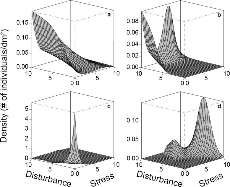
Figure 2 Contrasting responses of four species to stress and disturbance. Species A) is a ruderal and C) is a competitor, while species B) and D) cannot be assigned to a specific strategy. Species B) has two maxima, however only one of them is supported by observed data and the other is an extrapolation. Species D) also has two maxima, but only the global maximum was considered. 

The predicted density maximum for each model was used as indicator of stress and disturbance conditions that yield species maximum abundance and, thus, as coordinates for stress and disturbance tolerance in the strategy space. We will refer to these coordinates as maximum abundance coordinates (MAC; See Appendix 1 for MACs and attributes of all species).

To determine if MACs were related to categorical plant traits (life history, storage organs and life form), we conducted multivariate analyses of variance (MANOVA). In each analysis, stress and disturbance tolerances were incorporated as the response variables. In the cases where the MANOVA was significant, two ANOVAs were conducted, one using disturbance only and the other using stress only. This allowed us to determine if tolerance to stress or disturbance (or both) was associated to the target trait. The relationship between seed mass and MACs was analyzed by regressing seed mass on disturbance tolerance and stress tolerance. A GAM was used for this purpose. All statistical analyses were performed in R versions 3.0.2 and 3.1.3 (R Core Team 2015). GAMs and surface plots were performed with the mgcv (^{Wood 2004}) and rgl (^{Adler & Murdoch 2014}) libraries respectively.

Results

Allocation of species. Stress and disturbance had different effects on the density of each species (Figure 2). Despite this, the maximum abundance coordinates (MAC) of some species could be the same. This was the case for five species that had zero stress tolerance but had the largest possible tolerance to disturbance (bottom right corner in Figure 3). Some studied species could tolerate high intensities of both stress and disturbance. Thus, not all the species were restricted to the theoretical triangular area of the strategy space (Figure 3). Using log-linear analyses, we found that MACs were more common where the stress was low (χ² = 26.61, p < 0.0001, Figure 4A), whereas few MACs occurred at low disturbance levels (χ² = 17.64, p = 0.0001, Figure 4B). The interaction between both tolerances (stress and disturbance) did not affect the frequency of MACs in different portions of the strategy space (χ² = 4.91, p = 0.2961).

Figure 3 Stress and disturbance conditions where the 50 studied species attain maximum abundance. 

Figure 4 Frequency of species that attain maximum abundance under different stress (A) and disturbance (B) intensities. 

Life histories and functional attributes. All MANOVAs were significant (p < 0.05), indicating that the analyzed traits were related to the position of the MACs along the stress and disturbance axes. On average, annuals tolerated less stressful conditions (mean = 2.07) than perennials (mean = 3.69; p = 0.0493), but there were no significant differences in the disturbance tolerances of these groups of species. As expected, plants with storage organs tolerated more stress (mean = 5.08) than those without them (mean = 2.47; p = 0.0064). Again, there were no significant differences between the groups of plants in terms of disturbance.

Chamaephytes, geophytes, hemicryptophytes and therophytes only differed in their stress-disturbance tolerance when both variables were analyzed together (p = 0.0361) but not when the variables were analyzed separately. On average, chamaephytes reached maximum abundances under higher stress and disturbance intensities than any other plant group (mean MAC values for stress = 5.43, and disturbance = 6.79). Geophytes tolerated stress at low intensities and disturbance at intermediate intensities (stress = 3.34, disturbance = 4.66). Hemicryptophytes and therophytes tolerated low stress intensities (3.09 and 2.07, respectively) and high disturbance conditions (6.83 and 6.81, respectively).

The seed mass changed with the stress tolerance (p = 0.0165), but these effects were not found on the disturbance axis (p = 0.2088). Thus, the model was refitted using the stress tolerance as a unique predictor of the seed mass. The fitted model predicted maximum seed masses near an intermediate stress value (Stress = 4; Figure 5). This maximum seemed to be generated by a single species with an inordinately large mass, but the general pattern remained unchanged when that species was removed.

Figure 5 Effect of seed mass on stress tolerance (p = 0.0165). 

Discussion

This study proposes a novel strategy-allocation method that relies on the direct measurement of stress and disturbance levels, the two abiotic factors that define Grime’s primary plant strategies. The allocation method captured the independent effects of both stress and disturbance, and it was capable of positioning species along the stress and disturbance axes. We found that the life cycle, presence of water storage organs, life form and seed mass had effects on the stress and/or disturbance tolerance. Most attribute patterns observed were in line with Grime’s predictions and previous reports in the literature, but some of them were also contradictory. Although our method only provides the positions of species relative to each other in the strategy space, we will discuss how it can be used to classify species into Grime’s main strategies using additional information.

Allocation of species in the strategy space. The available methods to infer plant primary strategies and thus allocate them in specific portions of the strategy space are based on plant functional traits (^{Grime 1974}, ^{Hodgson et al. 1999}, ^{Pierce et al. 2013}, ²⁰¹⁷), but this approach generates several problems that make the theory virtually irrefutable (^{Li & Shipley 2017}). Primary strategies are defined by the tolerance of species to stress and disturbance and not by the traits that make this possible. As a result, allocation methods based on functional traits cannot identify strategies according to Grime’s proposal. For example, it has been suggested that most ruderals are annuals with fast growth rates and high fecundity (^{Grime 1977}, ^{Müller et al. 2014}, ^{Yuan et al. 2016}); however, these are contingent properties of ruderality, while the essential property of ruderals is tolerance to disturbance. The use of multiple contingent properties may be more robust than the use of a single trait, but it does not necessarily guarantee the inference of essential ones (^{Robertson & Atkins 2018}). We must then correctly quantify stress and disturbance levels as environmental properties to further infer the evolutionary trade-offs that species may have to tolerate (^{Li & Shipley 2017}). On such a basis, we can infer strategies based on essential properties and then link them to contingent ones.

Considering stress and disturbance levels as environmental properties (e.g., temperature, drought and fires are all environmental phenomena) that act regardless of species responses requires their quantification at the habitat level, which is not an easy task. The approach developed here is inherently limited, as we only focus on the main agents of stress and disturbance at the study site, namely, water availability and livestock activity. Given the large number of variables that determine plant performance in nature, it is of paramount importance to identify key stress and disturbance factors; this can be done by choosing factors that overwhelm other limitations because of their importance or magnitude. In our study, hydric stress was chosen because water is an essential resource for plants (i.e., it cannot be replaced by other resources) and, thus, it is subjected to Liebig’s law of the minimum: when it is lacking, such as in shallow soils, it becomes the sole factor that determines plant growth (^{Tilman 1980}). Factor selection will then depend on the environment under study. However, the difficulties involved in measuring stress, disturbance and plant tolerance may lead to the use of indirect indicators, as we did in our study (e.g., soil depth, livestock droppings and plant population density, respectively), and to make this method reliable, these indicators must closely reflect the underlying variables.

The difficulty in generalizing across environments subjected to different forms of disturbance and stress is the disadvantage of not employing species traits as surrogates for tolerance. Traits provide universality, but if these surrogates are also used to define CSR strategies, then it is clear that testing the theory will be difficult. Our approach suggests that environmental variables can be linked with morphological or life history traits using field data. ^{Li & Shipley (2017)} also provided evidence for such a link using laboratory data. Thus, both methods can be used to test the theory and validate which traits can be used to estimate species tolerance under local conditions.

Despite its inherent difficulties, the allocation of species to strategies based on the stress and disturbance measurements as environmental properties, not as species traits, is the only way to unambiguously test the theory (^{Li & Shipley 2017}) and to identify Grime’s plant strategies (1977). In our case, our results offer a glimpse at how the species of a heavily grazed, semiarid grassland tolerate these factors.

Our method showed that the studied species exhibited a wide range of tolerances to stress and disturbance and that they occupy a large fraction of the strategy space. There was a trend for more species to attain their maximum density under low stress but high disturbance conditions. Interestingly, some species tolerated both factors at high intensities, which is in agreement with ^{Herben et al. (2018)}, who recently showed that some species from sites with frequent disturbances and shallow soils, much like in our study system, occupied a region with high stress and disturbance in the strategy space. These findings may be due to the particular stress and disturbance combinations to which the plants are exposed.

Life history and functional attributes. ^{Grime (1977)} stated that each primary strategy has a set of morphological and physiological traits that result from evolutionary trade-offs. Therefore, certain attributes should be associated with either stress or disturbance tolerance. Stress-related traits followed the patterns expected from the theory. The same happened in terms of disturbance, although the relationships were not always significant. The exception was with Raunkiaer’s life forms, where the trends were more complex than anticipated. These results suggest that our indicators of stress and, to a lesser degree, disturbance are not off the mark and reflect the basic processes proposed in Grime’s theory.

In arid habitats, resources are often scarce and are available at pulses after long periods of shortage (^{Schwinning & Sala 2004}). Stress tolerance as a primary strategy has been identified as a conservative scheme in which the resources available during the pulses are stored for later use (^{Chaves et al. 2002}). As a result, several strategies for stress tolerance are possible, of which two were tested here: (1) maintaining longer life cycles (^{Grime 1977}, ²⁰⁰⁶) and (2) having water storage organs (^{Hanscom & Ting 1978}, ^{Osmond et al. 1987}, ^{Ogburn & Edwards 2010}).

The seed mass was not associated with the disturbance tolerance, and it had a complex relationship with stress (Figure 5). At low stress intensities, a positive relationship between tolerance and the seed mas was found, but the opposite occurred at high stress levels (above a stress value of 4; i.e., below 11 cm of soil depth). This result shows that seed traits may influence the stress tolerance, but a clear trade-off is difficult to discern. The annual life cycle is a hallmark trait of ruderal plants (^{Grime 1977}, ^{Müller et al. 2014}, ^{Yuan et al. 2016}), and, as expected, the abundance of therophytes increased at sites with low stress and high disturbance levels. ^{Grime (1977)} and others (^{Lavorel et al. 1999}, ^{Louault et al. 2005}, ^{Díaz et al. 2007}) provided evidence that plants with meristems closer to the ground are better protected against disturbance, especially that caused by grazers. In agreement with this, we found that hemicryptophytes (i.e., plants whose meristems are located in contact with or very close to the ground) tolerated high disturbance intensities, but the same was true for chamaephytes, which had the highest meristem position of all the perennial species studied. Geophytes did not follow the expected trend either, as their abundance increased at low disturbance intensities in spite of having subterranean meristems that could promote tolerance to disturbance (^{Gómez-García et al. 2009}). At our study site, however, there is some evidence that geophytes are strong competitors (^{Martorell et al. 2015}), and as such their maximum abundances should occur under low stress and disturbance conditions.

These results suggest that our basic approach can be reliably used to allocate species in the strategy space and that it is consistent with Grime’s proposal. The fact that some of our predictions about the relationship between disturbance tolerance and traits were not supported may reflect the inaccurate measurement of disturbance rather than a flaw in the general conception of the method. Disturbance was measured through a set of indirect indicators, such as livestock-dropping densities and distances to populated areas. Actual measurements of the stocking rates observed in each plot may succeed in producing a better estimate of the disturbance tolerance. We also neglected other factors involved in biomass reduction, such as grazing by invertebrates and lagomorphs. This limitation highlights the need to use proper stress and disturbance indicators.

Classification based on Grime’s strategies. In its current form, our method is able to determine which species are more ruderal, competitive or stress tolerant than others, but it cannot be used to determine if a species follows a given strategy. Two considerations may be helpful for this issue: the ranges of stress and disturbance values observed in the field and additional information regarding the biology of species or their attributes. For the first method, it is important to consider whether extreme values are observed. As we have discussed, our stress gradient included the most extreme value, so the plants that were ranked at high levels of disturbance tolerance can safely be considered stress-tolerant species. As an example of the second method, consider that half of the studied species with disturbance tolerance values higher than 5 are listed in the Mexican Weeds Database (^{Vibrans 2012}). Because weeds are a canonic example of ruderal plants (^{Grime 1977}), it would appear that species with high disturbance tolerances in our study should be classified as ruderals themselves.

Note that some species rank at high levels of both stress and disturbance tolerance. These species cannot be classified into any of the three primary strategies or their combinations, but they may belong to a fourth category whose existence has been discussed in previous works (^{Van der Steen & Scholten 1985}, ^{Grime 1988}, ^{Loehle 1988}, ^{Herben et al. 2018}).

Approaches such as that described here may be better equipped than traditional methods to test the three-primary-strategy theory and can aid in establishing the direct relationships between environmental conditions and species’ responses to them. Our method represents an initial step in tackling these complex tasks. Future refinements to these approaches will ultimately strengthen the underlying framework of Grime’s landmark theory.