


 texto en
  Inglés (pdf)
 Artículo en XML
 Referencias del artículo
 Enviar artículo por email
 Citado por SciELO
  Similares en
SciELO
Similares en
SciELO 
 Permalink
Introduction
The procedure described in the FAO-56 Manual is the most widely used to calculate crop evapotranspiration (ETc), which is the product of a crop coefficient (Kc) by reference evapotranspiration (ET0) (Allen et al., 2006). Wright (1982) proposed the dual method, where Kc is the product of the crop basal coefficient (Kcb) and the coefficient associated with soil evaporation (Ke). The Kcb component represents crop evaporation conditions under conditions where the soil surface is dry (direct evaporation from soil surface is minimal), and crop growth is not limited by water stress, phytosanitary, climatological or physiological factors (Rocha et al., 2011). Currently, Kcb is widely used to estimate actual evapotranspiration, which represents the potential baseline Kc value (Allen et al., 2006). The main reference on this subject is the FAO-56 Manual compendium; however, it has certain limitations, because it only provides Kcb values at three main stages for each crop and under standard conditions, which are non-existent in true applications (Mhawej et al., 2021).
The crop coefficient methodology is used to estimate ETc and schedule irrigation (Escarabajal et al., 2015). However, its application calls for the determination of Kcb for each crop and stage of development, which requires a variety of methods, many of which are time-consuming, destructive, and expensive in terms of time and money. For this reason, it has been decided to simplify their determination using variables such as leaf area index (Kirk et al., 2009), plant cover fraction (López-Urrea et al., 2009) or crop canopy reflectivity (Neale et al., 1989), among others.
The empirical relationship between biophysical variables and Kcb with vegetation indices is increasingly used due to the wide availability of remote sensing information (Odi-Lara et al., 2013). Currently, there are several equations or algorithms estimating Kcb for herbaceous crops (maize, wheat and grapevine, among others) using vegetation indices, such as the normalized difference vegetation index (NDVI) and the soil-adjusted vegetation index (SAVI), which are the most widely used because they are easy to calculate and derivable from a multispectral sensor (Candiago et al., 2015). Remote sensing allows estimations of large areas since they provide reliable spatial and temporal information over the crop growth period (Chaudhary & Srivastava, 2021).
Satellites have aroused great interest in the scientific community due to their multiple applications and high spatial, temporal, spectral and radiometric resolution (Borràs et al., 2017). The most widely used are those that provide free and easily accessible information, such as the Sentinel-2 satellite. In addition, satellite imagery, combined with geographic information technologies, are used with the objective of optimizing agricultural productivity, by considering spatial variability, as it is associated with each production plot (Lizarazo-Salcedo & Alfonso-Carvajal, 2011).
The Lagunera Region, where irrigation district (RD) 017 is located, is one of the main dairy basins at the national level, and livestock is fed mainly alfalfa, silage and concentrates. Maize silage is the most common, as it can account for 30 to 40% of the diet (on a dry basis) of production cows (González-Castañeda et al., 2005). Maize silage is a crop with high productivity, low protein content and good energy value (Núñez-Hernández et al., 2003). This has led to an increase in the areas planted with this crop, since it is also one of the forages that require less water (Arreola et al., 2016). In the last four years, this has been the main crop in the region, with a current area of 54 000 ha (Reyes-González et al., 2022), out of a total irrigated area of 167 000 ha.
The region has two sources of water for crop irrigation: surface water (river water) and groundwater (well water), but both sources are limited and have low availability. This situation forces producers to implement strategies to increase the efficient use of irrigation water, such as canal rehabilitation, pond construction, land leveling, and land irrigation technification, among others. However, all these efforts will not give the best results if they do not start from the principle of applying only the water requirements of the crops. Therefore, it is essential to make practical and operative estimates of Kcb throughout the growing season, to later calculate ETc and schedule irrigation with an efficient use of water.
The use of spectral information from Sentinel-2 satellite imagery is an alternative to the FAO-56 method to calculate Kcb. Therefore, the objective of this study was to evaluate nine algorithms (six using NDVI and three using SAVI) to estimate the Kcb of forage maize during the whole vegetative cycle in two plots with different water sources and different irrigation management. The algorithms with the best accuracies were identified when compared with the Kcb derived from tables in the FAO-56 Manual (Allen et al., 2006).
Materials and methods
The study was conducted during the spring-summer 2021 cycle in two forage maize plots located in the municipality of Francisco I. Madero, Coahuila, Mexico. Both plots are part of the irrigated area of Module XII of DR 017 Región Lagunera (Table 1; Figure 1). The climate is dry warm desert, with rainfall in summer and cool winter. Average annual rainfall is 258 mm and average annual evaporation is 2 000 mm, so the precipitation – evaporation ratio is 1:10. The average annual temperature is 21 °C, with a maximum of 33.7 °C and a minimum of 7.5 °C (García, 2004).
Table 1. Geographical location, planting and harvesting dates, and main characteristics of the study plots.
| Characteristics | Plot 1 | Plot 2 |
|---|---|---|
| Latitude | 25° 46’ 44.86” N | 25° 47’ 17.44” N |
| Longitude | 103° 18’ 48.65” O | 103° 18’ 15.96” O |
| Hybrid | N83N5 (SYNGENTA) | 8576 (ABT) |
| Sowing date | February 26, 2021 | April 09, 2021 |
| Harvesting date | June 28, 2021 | August 09, 2021 |
| Water source | Surface and Groundwater | Surface |
| Irrigated area (ha) | 11.41 | 6.32 |
| Irrigation system | Alphaliferous Valves | Gravity |
| Predominant soil texture | Silty clay loam | Clay |
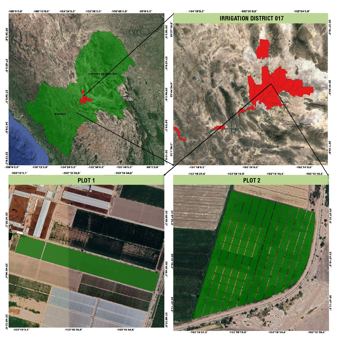
In both plots, seven seeds per linear meter were sown, with a row spacing of 0.76 m; this resulted in a sowing density of about 92 thousand plants∙ha-1. In Plot 1, five irrigations were applied: one pre-planting irrigation and four auxiliary irrigations. This property has surface (river) and groundwater (well) rights. The pre-sowing irrigation and the first auxiliary irrigation were applied with well water, and river water was used for the rest of the irrigation. In Plot 2, only surface water was used, and a pre-planting irrigation and two auxiliary irrigations were applied during the vegetative cycle.
Download and processing of satellite imagery
Twenty-six multispectral images from the cloud-free Sentinel 2A and 2B satellites were used, which satisfactorily covered the maize vegetative cycle in the two study plots. These satellites provide radiometric data through 13 bands: four spectral bands with a spatial resolution of 10 m, six of 20 m, and three of 60 m; at a temporal resolution of five days. The images were downloaded for free from the Copernicus Open Access Hub website (https://scihub.copernicus.eu/dhus/#/home), in GeoTIFF format and a typical compression of 950 MB per image. Orthorectified and atmospherically corrected images were downloaded, with processing level 2A, in which reflectance values are corrected for distortion caused by aerosols and atmospheric water vapor.
Subsequently, the polygons of interest in both plots were cut out using the freely available QGis v. 3.10.6 (2020) program. For this purpose, one melga per plot was selected. The melga in Plot 1 was 125 m long and 20 m wide, while the melga in Plot 2 had the same width but was 290 m long. Consequently, the study areas were 2 500 and 5 800 m2, respectively.
Estimating NDVI and SAVI indices
To estimate the Kcb of forage maize using remote sensing with the algorithms mentioned in Table 2, it is necessary to estimate the vegetation indices (NDVI and SAVI).
NDVI (Rouse et al., 1974) was calculated with Equation 1, for each scene in the area of interest.
where NDVI is the normalized difference vegetation index (dimensionless), NIR is the reflectance in the near infrared band (%) and R is the reflectance in the red band (%). According to the spectral bands included in the Sentinel-2 imagery; B8 corresponds to the NIR band and B4 to the R band, both with a spatial resolution of 10 m.
The SAVI index (Huete, 1988) was calculated using Equation 2:
Where L is a soil brightness correction factor, which minimizes the influence of soil on canopy reflectance, and therefore varies inversely according to the quantity of vegetation present (Qi et al., 1994). Therefore, in soils with vegetative development, the L factor is considered as zero, and the SAVI becomes equivalent to the NDVI equation. For this study, in the two plots, L values from 0.10 to 0.30 were used during the first 50 days after sowing (DAS) for Plot 1 and 63 DAS for Plot 2. In both plots, the value of zero was used for the rest of the cycle, because at this stage the crop had higher vegetative cover.
Measures of central tendency (mean and mode) of the aforementioned indexes were estimated at the melga level using the “Zonal Statistics” plug-in (installed in QGis v. 3.10.6). These values were compared with the values of maize Kcb tables provided by the FAO-56 Manual (Allen et al., 2006).
Preparation of the maize Kcb curve
For the elaboration of the Kcb curve of forage maize, the tables of the FAO-56 Manual (Allen et al., 2006) were consulted, where the Kcb values were selected at the initial (Kcb ini), middle (Kcb mid) and final (Kcb fin) stages (0.15, 1.15 and 0.50, respectively). The Kcb fin corresponds to the condition when the crop is harvested with a high percentage of moisture in the grain or for forage, as was the case. The Kcb values in tables are for sub-humid climates, with minimum relative humidity (RHmin) of 45 % and wind speed (VV) of 2 m∙s-1. Therefore, an adjustment was made to the Kcb in the two study plots based on the methodology described in the FAO-56 Manual (Allen et al., 2006). In Plot 1, Kcb values of 1.18 and 0.52 were determined for the middle and final stages, respectively. For Plot 2, the same Kcb values from tables were used for all growth stages since there were no differences between the adjusted Kcb and tables Kcb.
Growth stage lengths of forage maize were determined using the tables in the FAO-56 Manual (Allen et al., 2006). Also, the phenology of the crop was recorded in the field, the degree days of development (DDD) and the leaf area index (LAI) were estimated to complement the Kcb curve of the crop of interest. The residual method (Equation 3) was used to calculate DDD (Snyder, 1985). The base temperature used was 10 °C, and the maximum temperature was 30 °C; these values are the most used for maize crop (Hou et al., 2014). For maximum temperatures higher than 30 °C, these were taken as equal to 30 °C.
Where Tmax is the maximum temperature recorded on a specific day (°C), Tmin is the minimum temperature recorded on a specific day (°C) and Tbase is the species-specific base temperature.
LAI (m2∙m-2) was estimated indirectly in the two study plots using the relationship proposed by Kross et al. (2015) (Equation 4).
Estimating basal crop coefficient (Kcb) with vegetation indices
A total of nine algorithms were used to estimate the Kcb of forage maize (Table 2). According to the literature, six algorithms were developed for forage maize, and the rest for wheat (Equation 6) and grapes (Equation 9), considered as herbaceous crops like maize. To employ Equations (10), (13) and (15), the soil line (NDVImin and SAVImin) separating the bare soil surface with vegetation was calculated (Rukhovich et al., 2016). The soil line was obtained by simple linear regression of the red band R (independent variable) and near infrared NIR (dependent variable), using only pixels within the plots. At first, linear regression was carried out on the 26 images downloaded from the Sentinel-2 satellite, which fully cover the phenological cycle of forage maize from the two study plots. The image of April 02, 2021, had the highest R2 value (0.88), and its relationship is shown in Equation 5:
Where 1.308 represents the slope and 56.07 is the ordinate to the origin.
Table 2. Algorithms used to estimate Kcb of forage maize using vegetation indices (IV).
| Algorithms | IV | Equation | Source | |
|---|---|---|---|---|
| Choudhury KcbNDVI | NDVI | (6) |
|
Choudhury et al. (1994) |
| Glez-Piqueras KcbNDVI | NDVI | (7) |
|
González-Piqueras et al. (2005) |
| Calera y Glez KcbNDVI | NDVI | (8) |
|
Calera y González (2007) |
| Campos KcbNDVI | NDVI | (9) |
|
Campos et al. (2010) |
| Argolo KcbNDVI | NDVI | (10) | Argolo et al. (2020) | |
| Allen FAO-56 KcbNDVI | NDVI | (11) |
|
Allen et al. (2006) |
| (12) |
|
|||
| Glez-Dugo KcbSAVI | SAVI | (13) |
|
González-Dugo et al. (2009) |
| Glez-Piqueras KcbSAVI | SAVI | (14) |
|
González-Piqueras et al. (2005) |
| Argolo KcbSAVI | SAVI | (15) |
|
Argolo et al. (2020) |
Kcmax = mid-stage maize crop coefficient; NDVImax = maximum NDVI value of the scene; NDVImin = NDVI value at the soil line (0.10); n = coefficient related to crop leaf architecture, for NDVI the value of 0.5 is assumed and 1.0 for SAVI; fceff = fraction of effective soil cover (0.80); SAVImax = maximum SAVI value of the scene; SAVIsuelo or SAVImin = bare soil value (0.12).
With this relationship, and with the QGis v. 3.10.6 program plug-ins (“RasterDataPlotting” and “QuickWKT”), the NDVImin (0.10) and SAVImin (0.12) soil lines were determined.
Linear Equations (11) and (12) were obtained by simple linear regression between the average NDVI of the two study plots (delimitation by melga) and the value of Kcb from tables of the FAO-56 Manual. Both equations were fitted with ordinate to the origin at the null coordinates. Equation (11) was used to estimate the Kcb of forage maize in Plot 1 and Equation (12) was used for Plot 2.
To understand the spatial and temporal distribution of estimated Kcb in the two study plots, usable soil moisture depletion was determined by gravimetric moisture content sampling before and after each irrigation event.
Statistical analysis
To evaluate the precision of the estimated Kcb of forage maize compared to the Kcb of tables in the FAO-56 Manual, three statistical indicators were used: 1) coefficient of determination (R2), which reflects the goodness of fit of a model to the variable it seeks to explain (Equation 16); 2) mean squared error (MSE), which measures the variation of the values estimated compared to the observed ones (Equation 17), and 3) average relative error (ARE), which indicates in percentage of the approximation of the value estimated compared to the real value, the lower the value the better the approximation (Equation 18).
where yiobt are the Kcb data from FAO-56 Manual tables, (
Results and discussion
Growth stages of forage maize, as determined by tables of the FAO-56 Manual, are shown in Table 3. For both plots, the vegetative cycle was 122 days. Harvesting was carried out when the crop reached 34 and 35 % dry matter in Plot 1 and Plot 2, respectively; that is, when the maize was in the R3 and R4 stages of development, and the grain was identified in a milky state in Plot 2 and in a pasty state in Plot 1. Núñez-Hernández et al. (2005) recommends harvesting at 28 to 35 % dry matter to promote good fermentation during the maize silage process. In addition, in this range, forage losses during harvesting are minimal.
Table 3. Length of growth stages and phenology of the forage maize crop.
| Plot 1 | Plot 2 | ||||||||
|---|---|---|---|---|---|---|---|---|---|
| Kcb ini | Kcb dev | Kcb mid | Kcb fin | Kcb ini | Kcb dev | Kcb mid | Kcb fin | ||
| Stage length (days) | 31 | 51 | 30 | 10 | 31 | 51 | 30 | 10 | |
| Crop phenology | VE-V4 | V4-VT | VT-R3 | R3-R4 | VE-V5 | V5-V8 | V8-R2 | R2-R3 | |
| Cumulative DDD (°C) | 312.9 | 945.9 | 1 376.1 | 1 526.1 | 393.3 | 1 128.7 | 1 572.3 | 1 722.6 | |
| Leaf area index (m2∙m-2) | 0.0 | 3.0 | 5.1 | 3.2 | 0.0 | 2.7 | 4.9 | 2.6 | |
Kcbini = basal coefficient initial stage; Kcbdev = basal coefficient developmental stage; Kcbmid = basal coefficient middle stage; Kcbfin = basal coefficient final stage; DDD = degree days of development; VE-V4 = from emergence to vegetative stage with fourth leaf; V4-VT = from vegetative stage with fourth leaf to panicle; VT-R3 = from panicle to reproductive stage with milky grain; R3-R4 = from reproductive stage with milky grain to reproductive stage with doughy grain; VE-V5 = from emergence to vegetative stage with the fifth leaf; V5-V8 = from vegetative stage with the fifth leaf to vegetative stage with the eighth leaf; V8-R2 = rom vegetative stage with the eighth leaf to reproductive stage with granulation; R2-R3 = from reproductive stage with granulation to reproductive stage with milky grain.
A difference of 196.5 DDD at the final stage of crop growth (Kcb fin) was recorded between the two plots, with Plot 2 accumulating the largest amount of thermal energy. This depends on the sowing dates and geographic location of the plots, but also on irrigation management, which influences water availability and affects temperature, which decreases both water and thermal stress. Thus, forage maize is especially sensitive at the grain filling stage (Zhu & Burney, 2022). Núñez-Hernández et al. (2005) reported a value of 1 470 DDD, accumulated in 103 days of vegetative cycle of a forage maize hybrid evaluated in the same study area.
LAI of Plot 1 was higher than that of Plot 2 from the development stage (Kcb dev) to the final stage of the crop (Kcb fin), which is due to the higher number of irrigations and better distribution of these in Plot 1, resulting in lower depletion of available soil moisture (ASM) (Figure 2) and, consequently, lower water stress. Higher water stress has an impact on lower foliage production per unit area and lower biomass accumulation due to lower photosynthetically active radiation interception, which eventually leads to lower yield (Song et al., 2019). Montemayor-Trejo et al. (2007) reported maximum IAF values of 3.4 at 78 DAS of forage maize (development stage), in Comarca Lagunera, Mexico, when gravity irrigation was applied. However, in another study conducted in the same region, maximum values of IAF of 5 were reported in this same crop, values similar to those found in this study, but with drip irrigation (Montemayor-Trejo et al., 2012).
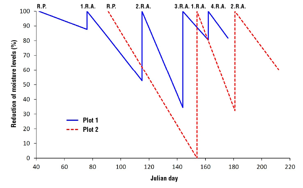
Figure 2. Temporal distribution of available soil moisture (ASM) depletion of the two study plots. RP = pre-sowing irrigation; RA = relief irrigation
Figure 2 shows the ASM of the soil profile determined by gravimetric moisture content sampling before and after irrigation, and average values of available moisture at a depth of 120 cm (15.4 % for Plot 1 and 13.5 % for Plot 2). Plot 2 showed the highest ASM (0 %) before applying the first relief irrigation (1.R.I.), which was applied 63 days after applying the pre-sowing irrigation (R.P.) and at 55 DAS. The programming of DR 017 is based on the requirements of the cotton crop, but it is not suitable for forage maize, which is reflected in low yields and low forage quality. In Plot 1 the highest ASM (34 %) was observed before 3.R.I., which was applied 29 days after 2.R.I. The rest of the irrigations, in both plots, were applied between 88 and 53 % of the ASM of the soil. The consumption of 50 % of available moisture is the optimum criterion for applying gravity irrigation to the study plots.
Table 4 shows the comparison of the Kcb estimated by the algorithms used in this study and the Kcb reported in the FAO-56 Manual during the initial, development, middle and final stages of the forage maize crop established in Plot 1. It is observed that the measure of central tendency showing lower values of error in the estimation of Kcb in all the algorithms used was the average at the melga level. Also, the Campos KcbNDVI algorithm had the lowest MSE value, both at the initial stage (Kcb ini) and at the development stage (Kcb dev). With reference to the middle stage (Kcb mid), the Glez-Dugo KcbSAVI algorithm had the lowest MSE value, and for the final stage (Kcb fin) it was the Glez-Piqueras KcbNDVI algorithm. When considering the four growth stages of forage maize, the Allen FAO-56 KcbNDVI and Argolo KcbSAVI algorithms showed the lowest MSE values. However, the Campos KcbNDVI algorithm presented, in each of the growth stages, values lower than 22 % of ARE, and in the whole vegetative cycle a ARE of 11.6 %, reaching an accuracy of 88.4 %. The above is satisfactory for estimating ETc using vegetation indices, since, according to Alfieri et al. (2017), an accuracy of 80 % is required.
Table 4. Comparison of the Kcb calculated by the algorithms and Kcb obtained from the FAO-56 Manual during the growth stages of forage maize grown in Plot 1.
| Algorithms | MCT | Kcbini (n = 6) | Kcbiev (n = 7) | Kcbmid (n = 6) | Kcbfin (n = 2) | Kcbcycle (n = 12) | ||||||||||
|---|---|---|---|---|---|---|---|---|---|---|---|---|---|---|---|---|
| MSE | ARE | MSE | ARE | MSE | ARE | MSE | ARE | R2 | MSE | ARE | ||||||
| Choudhury KcbNDVI | AVG | 0.26 | 170.8 | 0.20 | 29.5 | 0.10 | 8.2 | 0.29 | 29.6 | 0.92 | 0.21 | 19.6 | ||||
| Glez-Piqueras KcbNDVI | AVG | 0.20 | 134.2 | 0.14 | 19.3 | 0.17 | 14.2 | 0.12 | 1.5 | 0.92 | 0.18 | 9.9 | ||||
| Calera y Glez KcbNDVI | AVG | 0.21 | 139.8 | 0.13 | 16.9 | 0.20 | 16.7 | 0.21 | 17.5 | 0.92 | 0.18 | 7.9 | ||||
| Campos KcbNDVI | AVG | 0.04 | 8.3 | 0.06 | 2.9 | 0.26 | 22.2 | 0.17 | 8.8 | 0.92 | 0.16 | 11.6 | ||||
| Argolo KcbNDVI | AVG | 0.10 | 63.9 | 0.17 | 23.7 | 0.47 | 39.5 | 0.21 | 18.1 | 0.87 | 0.28 | 33.6 | ||||
| Allen FAO-56 KcbNDVI | AVG | 0.10 | 59.5 | 0.10 | 13.6 | 0.16 | 13.2 | 0.24 | 21.9 | 0.92 | 0.14 | 4.0 | ||||
| Glez-Dugo KcbSAVI | AVG | 0.07 | 7.4 | 0.27 | 37.0 | 0.06 | 3.6 | 0.39 | 44.4 | 0.90 | 0.20 | 18.2 | ||||
| Glez-Piqueras KcbSAVI | AVG | 0.36 | 239.1 | 0.44 | 68.6 | 0.16 | 13.6 | 0.52 | 60.2 | 0.90 | 0.37 | 50.8 | ||||
| Argolo KcbSAVI | AVG | 0.07 | 25.9 | 0.09 | 9.6 | 0.21 | 17.1 | 0.20 | 15.5 | 0.90 | 0.14 | 5.5 | ||||
MTC = medida de tendencia central; Prom = promedio; R2 = coeficiente de determinación (adimensional); CME = cuadrado medio del error (adimensional); ERP = error relativo promedio (%); n = número de observaciones (imágenes satelitales utilizadas); Kcbini = coeficiente de cultivo basal inicial; Kcbdes = coeficiente de cultivo basal de desarrollo; Kcbmed = coeficiente de cultivo basal medio; Kcbfin = coeficiente de cultivo basal final; Kcbciclo = coeficiente de cultivo basal del ciclo.
Table 5 shows that the mode had lower MSE values in most of the algorithms used to calculate Kcb in Plot 2, except for the equations Campos KcbNDVI, Argolo KcbNDVI and Allen FAO-56 KcbNDVI. In these expressions, the average had lower MSE value. The Argolo KcbSAVI algorithm had lower MSE values in the Kcb ini and Kcb dev stages. For Kcb mid and Kcb fin stages, the lowest MSE value was with Choudhury KcbNDVI. However, when considering the whole maize growing cycle, the Argolo KcbSAVI algorithm had the lowest MSE value, but Argolo KcbNDVI algorithm had values lower than 13 % of ARE at the four stages of maize growth, and 8.3 % of ARE in the whole growing cycle, resulting in an accuracy of 91.7 %.
Table 5. Comparison of Kcb calculated by the algorithms and the Kcb obtained from the FAO-56 Manual during the growth stages of forage maize grown in Plot 2.
| Algorithms | MTCT | Kcbini (n = 3) | Kcbdev (n = 10) | Kcbmed (n = 3) | Kcbfin (n = 1) | Kcbcycle (n = 17) | ||||||||||
|---|---|---|---|---|---|---|---|---|---|---|---|---|---|---|---|---|
| MSE | ARE | MSE | ARE | MSE | ARE | MSE | ARE | R2 | MSE | ARE | ||||||
| Choudhury KcbNDVI | Moda | 0.31 | 202.8 | 0.14 | 13.3 | 0.05 | 0.7 | 0.03 | 3.2 | 0.92 | 0.17 | 15.6 | ||||
| Glez-Piqueras KcbNDVI | Moda | 0.25 | 165.4 | 0.12 | 3.4 | 0.09 | 7.0 | 0.04 | 3.4 | 0.92 | 0.14 | 6.0 | ||||
| Calera y Glez KcbNDVI | Moda | 0.26 | 169.2 | 0.12 | 2.0 | 0.12 | 9.9 | 0.07 | 6.3 | 0.92 | 0.15 | 4.2 | ||||
| Campos KcbNDVI | AVG | 0.19 | 98.9 | 0.15 | 19.5 | 0.09 | 7.3 | 0.04 | 3.5 | 0.94 | 0.15 | 12.3 | ||||
| Argolo KcbNDVI | AVG | 0.08 | 2.6 | 0.12 | 9.3 | 0.14 | 6.8 | 0.13 | 12.1 | 0.93 | 0.11 | 8.3 | ||||
| Allen FAO-56 KcbNDVI | AVG | 0.21 | 121.3 | 0.14 | 12.8 | 0.18 | 15.5 | 0.13 | 11.9 | 0.94 | 0.16 | 6.1 | ||||
| Glez-Dugo KcbSAVI | Moda | 0.12 | 52.8 | 0.14 | 13.6 | 0.19 | 14.7 | 0.20 | 18.5 | 0.95 | 0.15 | 16.0 | ||||
| Glez-Piqueras KcbSAVI | Moda | 0.43 | 285.3 | 0.33 | 50.9 | 0.27 | 23.1 | 0.30 | 27.9 | 0.95 | 0.34 | 49.5 | ||||
| Argolo KcbSAVI | Moda | 0.08 | 22.2 | 0.10 | 9.1 | 0.12 | 8.2 | 0.06 | 5.2 | 0.95 | 0.10 | 7.2 | ||||
MCT = measure of central tendency; AVG = average; R2 = coefficient of determination (dimensionless); MSE = Mean squared error (dimensionless); ARE = average relative error (%); n = number of observations (satellite images used); Kcbini = initial basal crop coefficient; Kcbdev = developmental basal crop coefficient; Kcbmid = mean basal crop coefficient; Kcbfin = final basal crop coefficient; Kcb cycle = cycle basal crop coefficient.
The Campos KcbNDVI algorithm had the lowest ARE values in the two plots studied, both by growth stage and in the whole vegetative cycle, except for Kcb ini and Kcb dev stages in Plot 2. Thus, this algorithm is reliable for estimating Kcb of forage maize with different surface irrigation management.
Figures 3 and 4 show the distribution of the calculated Kcb and the Kcb reported in the FAO-56 Manual of crop growth. In Plot 1 it is observed that in the Kcb ini and Kcb dev stages of the crop most of the algorithms overestimate Kcb. In the Kcb ini stage the algorithms overestimated Kcb from 60 to 239 %, and in the Kcb dev stage they overestimated Kcb from 10 to 69 %. In contrast, at the Kcb mid stage most algorithms underestimated Kcb from 4 to 40 %, and at the Kcb fin stage most overestimated Kcb from 2 to 60 %. Five irrigations were applied throughout the vegetative cycle of the crop, which were distributed in a pre-sowing or aniego irrigation, and four auxiliary irrigations applied at 19, 58, 87 and 105 DAS, with an accumulated gross irrigation lamina of 93.4 cm (Figure 3).
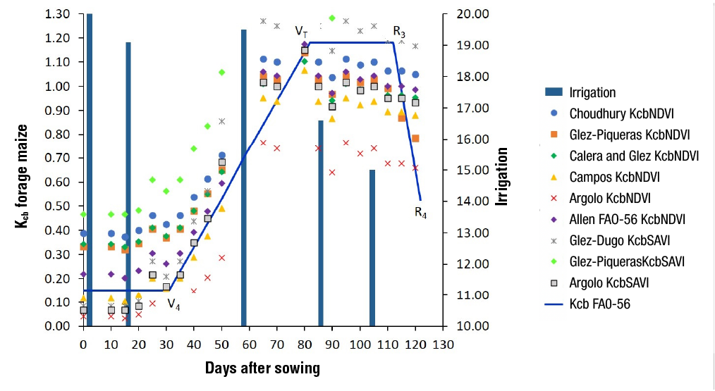
Figure 3. Distribution of Kcb estimated by the algorithms used and the Kcb obtained from the FAO-56 Manual of forage maize grown in Plot 1.
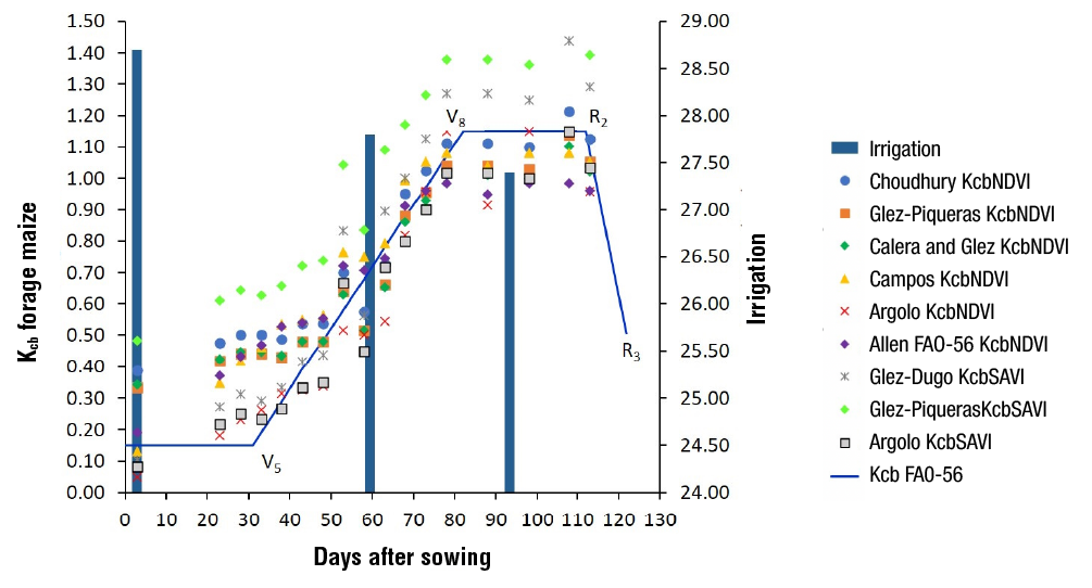
Figure 4. Distribution of the Kcb estimated by the algorithms used and the Kcb obtained from the FAO-56 Manual of forage maize grown in Plot 2.
In general, it was observed that in the two study plots the algorithms used had a lower adjustment in the initial and final periods of the crop. This is because the crop cover values are lower and soil evaporation, not considered by Kcb, has a greater effect (Allen et al., 2006), so there is greater variation in the daily values of Kcb ini and Kcb fin depending on the water status of the surface soil layer (Rocha et al., 2011).
Figures 5 and 6 show the Kcb maps generated with the Campos KcbNDVI algorithm in the two study plots at pixel scale. This algorithm had the best statistical indices when comparing the estimated Kcb with the Kcb from tables in the FAO-56 Manual. Plot 1 showed a Kcb variation from 0.13 to 0.32 in the initial stage (Julian day 77), from 0.25 to 0.59 in the development stage (Julian day 107), from 0.82 to 1.05 in the middle stage (Julian day 142) and from 0.77 to 0.96 in the final stage (Julian day 172) (Figure 5).
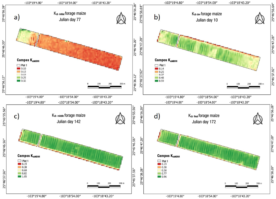
Figure 5. Spatial and temporal distribution of Kcb of forage maize grown in Plot 1 in the stages: a) initial (77 Julian day),
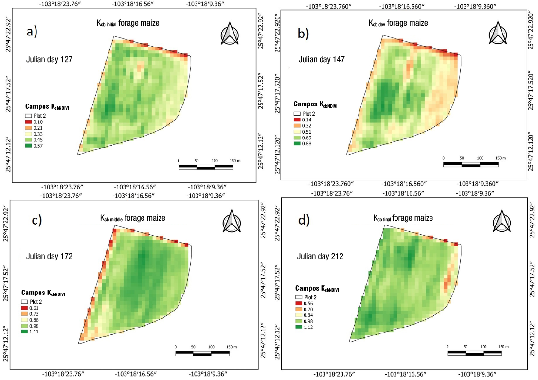
Figure 6. Spatial and temporal distribution of Kcb of forage maize grown in Plot 2 in the stages: a) initial (127 Julian day),
Plot 2 had Kcb variations from 0.33 to 0.57 in the initial stage (Julian day 127), from 0.32 to 0.88 in the development stage (Julian day 147), from 0.86 to 1.11 in the middle stage (Julian day 172) and from 0.70 to 1.12 in the final stage (Julian day 212) (Figure 6). It is observed that Plot 2 had greater variation in Kcb values in all growth stages of forage maize. This could be due to factors such as crop type (hybrid), soil texture, irrigation management or microclimate, individually or in combination. The maps allow to identify areas with irrigation stress or poor nutrition, irrigation system malfunction or other environmental stress (Knipper et al., 2019).
The Kcb estimated by the Campos KcbNDVI algorithm were similar to those reported by Gao et al. (2009) in two maize growth stages (initial and mid), with values from 0.36 to 0.37 in the Kcb ini stage, from 1.18 to 1.19 in the Kcb mid stage and from 0.22 to 0.28 in the Kcb fin stage. The values of the last stage were different from those reported in this study, since the first Kcb values concern maize for grain. Ojeda et al. (2006) obtained Kc values, using a model based on accumulated DDD, from 0.05 to 0.3 in emergence (VE), from 0.4 to 0.45 in vegetative stage with four leaves (V4), from 1 to 1.12 in panicle stage (VT), from 1.15 to 1.25 in reproductive stage with stigmas appearance (R1), from 1.1 to 1.2 in reproductive stage with granulation (R2), from 1 to in reproductive stage with milky grain (R3) and from 0.8 to 1 in reproductive stage with doughy grain (R4). Reyes-González et al. (2019) found Kcb values of 0.22 to 0.40 at the Kcb ini stage, 1.00 at the Kcb mid stage and 0.80 at the Kcb fin stage, in the same study area.
The Kcb derived from the spectral information of the Sentinel-2 images are independent from the parameters of time, sowing day and effective coverage, and represent the evolution of crops in quasi-real time. Hereby, the difference corresponds only to the time lapse in collecting the satellite imagery and processing the information (1-2 days), which facilitates irrigation scheduling in a large region, since neither sowing dates nor assumed effective coverage are required (Rocha et al., 2011).
Conclusions
The use of spectral information from the red and near infrared bands recorded in Sentinel-2 satellite imagery is a viable and adequate alternative to the FAO-56 Manual method for calculating the basal crop coefficient (Kcb) of forage maize. In addition, by combining the use of this technology with the collection of information in the field, it is possible to analyze its behavior more precisely and make more accurate estimates, as specific information is available for the crop cycle and study site. This makes it possible to monitor its evolution in quasi-real time and, consequently, to schedule irrigation in a convenient way in time and space, thus increasing the efficiency of water use.
The Campos KcbNDVI algorithm had the best accuracies for estimating the Kcb of forage maize in the two different conditions of field irrigation, both in its growth stages and in its entire crop cycle, obtaining an average accuracy of 88 %.

