


 texto en
  Inglés (pdf)
 Artículo en XML
 Referencias del artículo
 Enviar artículo por email
 Citado por SciELO
  Similares en
SciELO
Similares en
SciELO 
 Permalink
Introduction
Greenhouses in warm and temperate regions use natural ventilation as a method of microclimate control, although at certain times of the year it is difficult to maintain adequate temperature and humidity values for crop growth and development. Tamimi et al. (2013) mention that greenhouses can be mechanically ventilated and cooled by wet-wall and fogging systems, which use evaporative cooling to maintain the desired climate inside the greenhouse. A favorable internal environment can be achieved by evacuating excess heat during high insolation (Montero et al., 2001).
Evaporative cooling is the most efficient way to cool the environment inside a greenhouse, especially if the outside air is dry (Kittas et al., 2011). These systems are based on the conversion of sensible heat into latent heat through the evaporation of water, which is supplied mechanically (Arbel et al., 2003). Upon evaporation, water droplets extract thermal energy from the surrounding environment and decreases air temperature while increasing humidity levels (Tamimi et al., 2013). The advantage of fogging systems compared to wet-wall systems, is the uniformity of conditions throughout the greenhouse, so forced ventilation is not necessary (Kittas et al., 2011).
Computational fluid dynamics (CFD) efficiently develops solutions in spatial and temporal fields of pressure, temperature and fluid velocity, and has shown results in the design and optimization of systems within the chemical, hydrodynamic and aerospace industries (Norton et al., 2007). In recent years, CFD has been used to study climatic conditions inside greenhouses. Kim et al. (2008) developed a CFD model of humidity distribution in a greenhouse without plants and equipped with fogging system and dehumidifiers with fogging system. In this case, the errors of the simulations for relative humidity were from 0.1 to 18.4 % with fogging system and from 1.1 to 13.1 % with dehumidifiers and fogging system. Tamimi et al. (2013) developed a model to analyze air movement inside a naturally ventilated greenhouse equipped with fogging system. The model estimated temperature and relative humidity with an error of 5.7 to 9.4 % and 12.2 to 26.9 %, respectively.
Based on the above, the objective of this study was to develop a 3D CFD model to analyze the temperature and humidity distribution of a naturally ventilated greenhouse (equipped with mechanical humidifiers) with bell pepper (Capsicum annuum L.) crop, to provide a tool for the design and management of environmental conditions suitable for crop growth and development in greenhouses of the region.
Materials and methods
Greenhouse description
The study was conducted in a greenhouse at the experimental station “Cerona” of the Universidad Autónoma Chapingo, Chapingo, Estado de México (19° 29’ 04.1” N and 98° 53’ 08.9” W, at 2 244 m of altitude). Experimental tests were performed with humidification equipment with mechanical fans (hydrophanes) from March 7 to 25, 2014 to define the initial, boundary and validation values of the CFD model. The model was not calibrated, only validated. The complete process for the numerical simulation, using the commercial CFD code, was as follows: geometry generation, meshing, problem solving, model validation with experimental temperature and humidity data, and obtaining the results. The finite volume method was used, and the Piso algorithm was used to solve the Navier-Stokes flow equations (Fatnassi et al., 2006).
Humidifiers produce an air mass flow rate of 1.53 kg·s-1, with a volume per unit of 0.098 m3 and a water expenditure of 0.0224 kg·s-1. The fan generates an airflow velocity of 6.36 m·s-1 and a momentum of 99.2 N·m-3. The greenhouse had side windows and curved structure at the top; also, it was composed of three tunnels joined in battery with zenithal windows (Figure 1). The overall dimensions of the greenhouse were 27 m wide (9 m each tunnel), 93 m long and 7.6 m high (4 m height to the gutters), with a total covered area of 2 511 m2 and NE-SW orientation of the crossbar. During the experiment, the greenhouse was occupied by a bell pepper crop with a density of 2.9 plants·m-2 and leaf area index of 3.21 m2·m-2, with crop row width of 1 m, height of 2 m, and row of 1 m.

Thermo-physical properties of greenhouse, soil and crop materials were taken from Fidaros et al. (2010), Flores-Velázquez et al. (2011) and Piscia et al. (2012). The optimum temperature values were 23/18 °C for day/night, which are those required for the growth and development of the bell pepper crop.
Temperature, relative humidity, solar radiation, and wind speed and direction were the climatic variables evaluated. Measurements were taken in the central area of the greenhouse, at 20 points distributed along the longitudinal and transverse axis at different heights (1.5, 2.5 and 4 m above the floor). All variables were measured and stored every minute; two HMP60 and one HMP50 (Vaisala, USA) temperature and relative humidity sensors, nine 108-type temperature sensors and eight HOBO UX 100-003 temperature and relative humidity sensors were used for this purpose. Wind speed was measured with a sonic anemometer (WindSonic c1 RS-232 2D, Campbell Scientific®, USA), and solar radiation with a pyranometer (CMP3, Kipp and Zonen, The Netherlands). All sensors were connected to a data logger (CR1000, Campbell Scientific®, USA), except for the HOBO UX 100-003 sensors, because these sensors have an integrated data logger.
External environmental measurements were obtained from a weather station (HOBO U30, Onset Computer Corporation, USA) located at Chapingo, Mexico. These weather conditions were used as initial conditions in CFD simulations. A series of five tests per day were performed at intervals of 15 to 20 min, which was when humidifiers were operating. The experiment consisted of 15 min on and 15 min off, only during the hours of highest temperature. This procedure was chosen because this is the traditional way of using hydrophanes. The wind direction was considered perpendicular to the window located in the NE part of the greenhouse (Table 1). Wind speed and solar radiation data were taken every 15 min from the weather station located at the Universidad Autónoma Chapingo.
Table 1 Environmental variables external to the greenhouse for four days.
| 20/03/2014 | 21/03/2014 | 22/03/2014 | 25/03/2014 | |
|---|---|---|---|---|
| Time (HH:MM) | 14:05 | 14:00 | 11:50 | 13:50 |
| Test time (min) | 15 | 15 | 20 | 15 |
| Temperature (°C) | 23.16 | 26.45 | 23.5 | 25.55 |
| Relative humidity (%) | 42.8 | 27.9 | 35 | 28.5 |
| Specific humidity (kgH2O·kgair -1) | 0.009886 | 0.007835 | 0.008244 | 0.007587 |
| Solar radiation (W·m-2) | 698.1 | 551.9 | 763.1 | 939.4 |
| Wind speed (m·s-1) | 2.27 | 3.02 | 3.02 | 2.01 |
Statistical analysis
The statistical criteria used to evaluate the model results were root mean square error (RMSE) and mean absolute error (MAE):
where N is the number of observations, P denotes the predicted values and O denotes the observed values (Alexandris et al., 2006).
Temperature and humidity modeling with computational fluid dynamics
The commercial program ANSYS Workbench 14.5 was used for the development of simulations.
General equation of conservation of mass, quantity of motion and energy of a fluid
The motion of a fluid is based on physical processes that are formulated as a series of partial derivative equations to represent the laws describing the flow. Specially, if one considers the flow of a fluid (air) within the domain Ω ⊂ Rn during a time interval 0, t, the dynamics of the flow at each point x, and at the specific instant t, is determined by state variables, the mass density ρ(x, t), the velocity field u(x, t) and its energy e(x, t). These characteristics are included in the Navier-Stokes equations (Flores-Velázquez et al., 2011).
The CFD numerical technique solves the Navier-Stokes equations within each cell of the computational domain (Bournet et al., 2007). The program used can solve the continuity, momentum, and energy equations (steady state and transient state). Patankar (1980) describes the general transport equation in differential form, which is composed of four terms: transient, convection, diffusion, and source (Equation 3).
Where ρ is the flux density, u is the velocity field, ∇ is the nabla operator denoting the gradient, Γ represents the diffusion coefficient, S ϕ is the source term and ϕ is a form of dependent variable (it can be mass fraction of a chemical species, component velocity or temperature) and describes the flow characteristics at a point location at a specific time; in a three-dimensional space, it would be ϕ = ϕ (x, y, z, t).
Turbulence model
Ventilation flows are often associated with turbulent motion, primarily due to high flow rates and heat transfer interactions involved in the flow field (Norton et al., 2007). In this study, the standard k − ε turbulence model was used to solve k (turbulence kinetic energy, m2·s-2) and ε (dissipation rate, m2·s-3), because according to the literature, this model appropriately describes the nature of fluid flow in greenhouses (Piscia et al., 2012; Romero-Gómez et al., 2010). Such model uses the following transport equations for k and ε (Launder & Spalding, 1974; Patankar, 1980):
where u i is the component of velocity in the i direction (m·s-1), x i indicates the i direction, μ is the dynamic viscosity of air (kg·s-1·m-1), μ t is turbulent viscosity (kg·m-1·s-1), G k is turbulent kinematic energy production (kg·m-1·s-3) and G b is turbulent kinetic energy production due to buoyancy (kg·m-1·s-3). μ t , G k and G b were calculated with the following relationships:
where u’ i is the fluctuating velocity component in the i direction (m·s-1), β is the thermal expansion coefficient (K-1), Pr t is the turbulence Prandtl number (dimensionless) and g i is any field acceleration in the i direction (m·s-2, for this case only gravitational acceleration). The coefficients given by FLUENT for the standard k − ε turbulence model are used in all calculations and are as follows: C 1ε = 1.44, C 2ε = 1.92, C μ = 0.09, C 3ε = tanh [abs (v/u)], σ ε = 1.0 and σ ε = 1.3.
Buoyancy model
In accompanied heat transfer flows, the properties of fluids are usually in accordance with temperature. Temperature variations can be small and yet be the cause of fluid motion. Density is commonly assumed to vary linearly with temperature (Ferziger & Peric, 2002). In this sense, the buoyancy effect is adequately modeled with the Boussinesq approximation:
where ρ 0 (operating pressure, kg·m-3) and T 0 (air temperature, K) are constant reference values, and the coefficient of volumetric thermal expansion (β) can be calculated based on the ideal gas assumption:
Discrete ordinate radiation model
Almost all the energy for physical and biological processes on the earth's surface comes from the sun, and a large part of this energy is scattered or stored in thermal form (Monteith & Unsworth, 2013). First, solar radiation heats the greenhouse structure, which increases internal temperature; then, it is absorbed by the crop (Rojano et al., 2014). Global solar radiation contributes, to a large extent, to the transpiration of greenhouse crops (Boulard & Wang, 2002). The discrete ordinate radiation model was used (Rojano et al., 2014) to simulate the effect of solar radiation in this study.
where
Discrete phase model and species transportation
The discrete phase model was selected to analyze the change of the thermal environment from the formation of water particles sprayed by humidifiers. Thus, the trajectory of the sprayed droplets can be tracked, and their heat transfer can be analyzed (Kim et al., 2008). To estimate humidity, the species transport model was used to determine the mass conservation equation, which is necessary to calculate the mass fraction of water along the domain. This model also predicts the energy exchange between the continuous phase and droplets, according to an energy balance involving latent and sensible heat transfer (Tamimi et al., 2013). Such a model can be written (for the x-direction in Cartesian coordinates) as follows:
where F D (u − u p ) is drag force per unit mass of particles, u is the liquid phase velocity, u p is the particle velocity, ρ is the fluid density, ρ p is the particle density and F x is the additional force, which also includes forces on particles arising due to the rotation of the reference frame.
Model of porous media
In this study, both the culture and the insect screens were considered as porous media, which have been modeled in terms of permeability and porosity (Miguel et al., 1997). The equation for the movement of a fluid through a porous mesh can be derived from the Forcheimer equation.
where μ is the dynamic viscosity of the fluid (kg·m-1·s-1), K is the intrinsic permeability of the medium (m2), C F is the inertial factor (Y, also called nonlinear pressure drop coefficient), ρ is air density (kg·m-3), u is air velocity (m·s-1) and ∂x is thickness (e s ) of the porous material (m).
The geometric characteristics and parameters of the meshes used in the study were obtained from v − ∆P, curves, obtained from wind tunnel experiments, and correspond to the M3 Anti-aphid mesh (Pérez-Vega et al., 2016).
The presence of crop in a greenhouse affects the overall airflow patterns and is expressed as follows:
where C 1 = 1/K is the viscous drag (m-2), C 2 is the inertial drag (m-1) and v the fluid velocity (m·s-1). According to Tamimi et al. (2013), coefficients C 1 and C 2 are determined as follows:
where C f is a nonlinear momentum loss coefficient (dimensionless), LAD is 1.6 m-2·m-3 and C D is the drag coefficient.
Molina-Aiz et al. (2006) show that the value of C D obtained for tomato, bell pepper, eggplant and beans were similar, and that leaf shape and size are not significant. For that reason, several authors have adopted the value of C D = 0.32 (Ali et al., 2014; Boulard & Wang, 2002). In addition, from the methodology reported by Sase et al. (2012)C f can be determined. Therefore, the values considered for this study were as follows: C f = 0.153, C 1 = 14.79 m-2 and C 2 = 1.03 m-1.
Crop transpiration model
Evapotranspiration (ET) of greenhouse crops is a complex process that depends on several environmental factors such as solar radiation, humidity, temperature, and air velocity (Tamimi et al., 2013). ET was considered as a homogeneous and constant vapor source according to the environmental conditions inside the greenhouse and regarding the average of 20 points distributed on the transverse and longitudinal axis at different heights. The ET model used was the one proposed by Baille et al. (1994), which has given excellent results for greenhouse crops with plastic cover in the central region of Mexico (Ruiz-García et al., 2015). These authors decompose the ET rate into day (E d , kg·m-2·s-1) and night (E n , kg·m-2·s-1) using the following expressions:
where A is the radiative parameter, K e is the radiation extinction coefficient (0.70 dimensionless), LAI is the crop leaf area index, I sun is the global solar radiation (W·m-2), λ is the latent heat of vaporization of water (2 454 000 J·kg-1) and VPD is the vapor pressure deficit (Pa). Parameters A (0.32, dimensionless), B d (30.15 x 10⁻³ W·m-2·Pa-1) and B n (15.21 x 10⁻³ W·m-2·Pa-1) were taken from Ruiz-García et al. (2015).
Results and discussion
Transient-state air temperature of CFD simulations in a greenhouse with crop
The performance obtained with the CFD model, with respect to the data measured during 4 days of tests with humidification in intervals of 15 min time intervals, shows that the best adjustment was for the CFD model on March 21, 2014; this according to the MAE and RMSE statistical criteria (Alexandris et al., 2006). The best adjustment had an error of 0.09 at 2.05 °C, and the worst adjustment of 0.29 at 4.2 °C (Table 2). These results agree with those reported by Tamimi et al. (2013), who performed a CFD model of a naturally ventilated greenhouse with fogging system.
Table 2 Comparison of air temperature predicted by the 3D computational fluid dynamics model versus measurements inside the greenhouse.
| 03/20/2014 | 03/21/2014 | 03/22/2014 | 03/25/2014 | Overall average | |
|---|---|---|---|---|---|
| Measured temperature (°C) | 28.74 | 31.12 | 29.15 | 29.38 | 29.6 |
| Simulated temperature (°C) | 28.55 | 31.4 | 30.08 | 31.71 | 30.43 |
| Absolute error | 0.92 | 0.88 | 1.35 | 2.32 | 1.37 |
| Maximum error (°C) | 2.63 | 2.05 | 2.77 | 4.20 | 2.91 |
| Minimum error (°C) | 0.05 | 0.09 | 0.34 | 0.29 | 0.19 |
| Mean absolute error | 0.05 | 0.04 | 0.07 | 0.12 | 0.07 |
| Root mean square error (°C) | 1.20 | 1.07 | 1.49 | 2.49 | 1.56 |
The comparison between the experimentally measured data and their corresponding data taken from the CFD simulations at 20 distributed points shows an overestimation by the CFD model for the air temperature inside the greenhouse. The best adjustment was on March 21, 2014, and the worst was on March 25, 2014. The average air temperature at the 20 points used in the experimental and simulated data sets was 29.60 ± 1.09 °C and 30.43 ± 2.07 °C, respectively (Figure 2). These values agree with those reported by Tamimi et al. (2013), who obtained 28.1 and 28.2 °C, respectively.
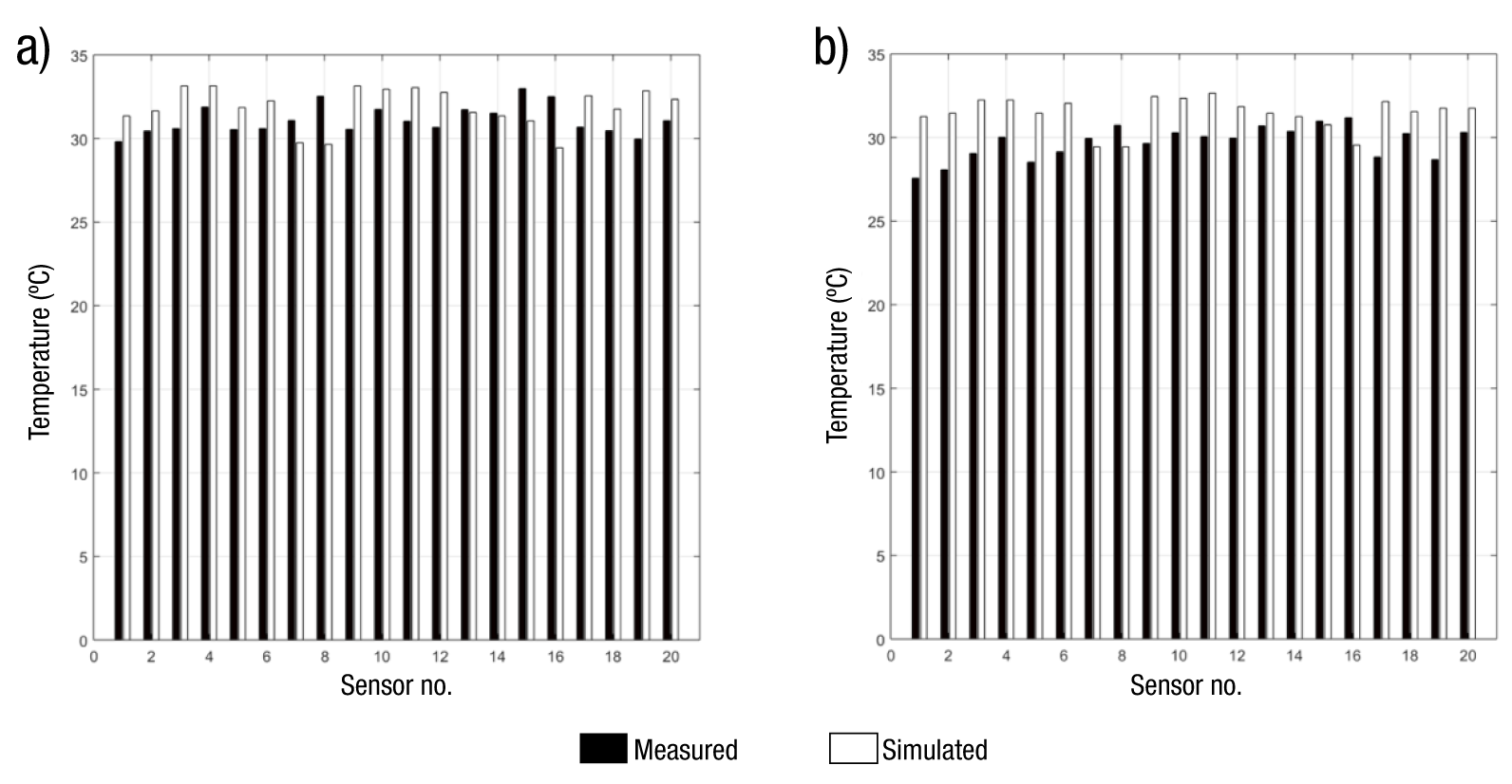
Figure 2 Comparison of measured (every 15 min) and simulated air temperature on 20 sensors located in the experimental greenhouse. Dates: a) 03/21/2014 and b) 03/25/2014.
The air temperature inside the greenhouse is modified by the action of the humidifiers, so a difference of 5 °C was recorded in the area above the crop and close to the hydrophanes. In addition, it was observed that the air temperature distribution strongly depends on the external environmental conditions, as well as on the wind direction (Figure 3).
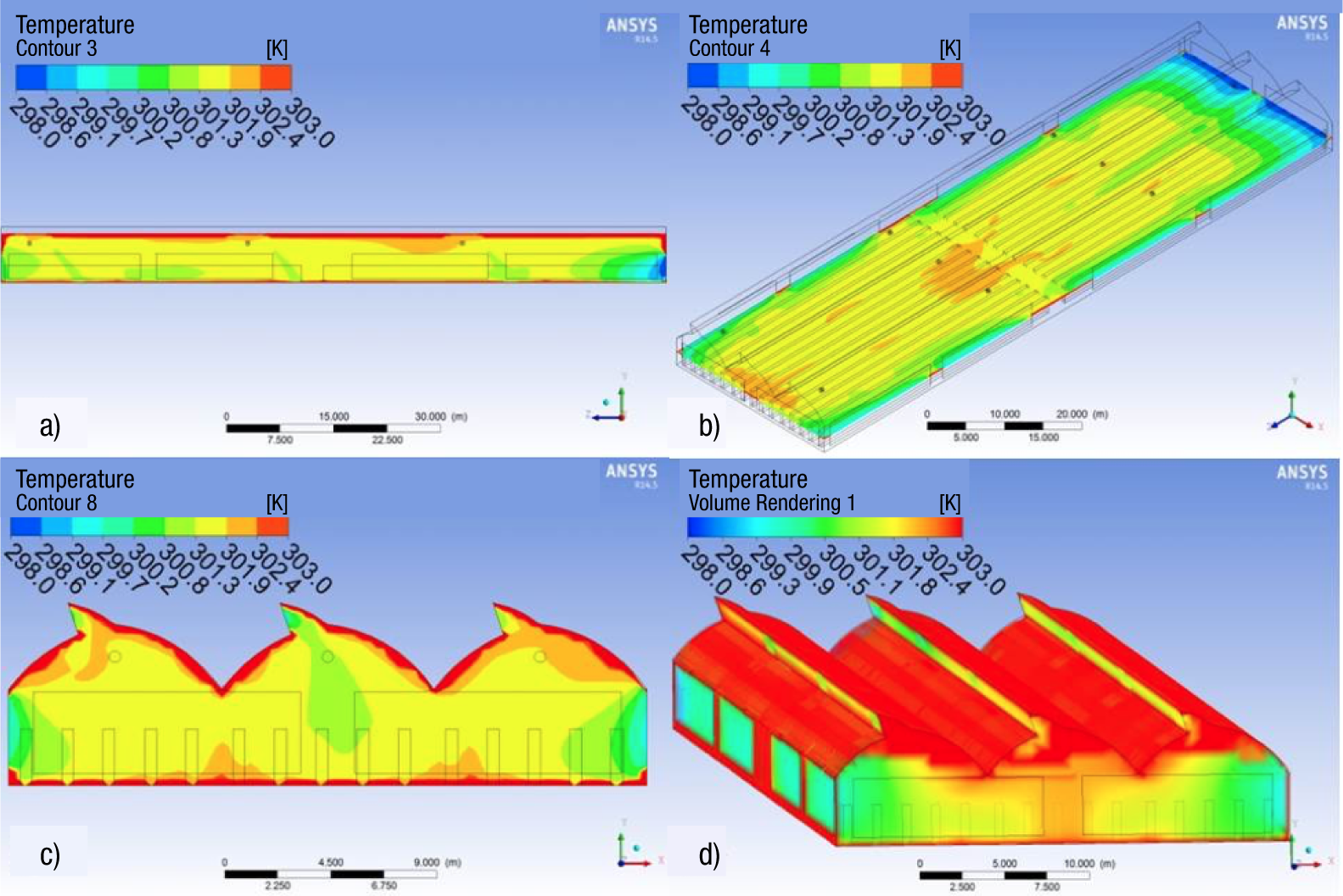
Figure 3 Air temperature distribution inside the greenhouse on March 20, 2014: a) side view in the central part of the greenhouse, b) top view 2 m above the ground, c) front view in the center of the greenhouse, and d) three-dimensional view of air temperature in the greenhouse.
Figure 3A shows that the indoor air temperature, close to the windows, is similar to the outdoor temperature of 24.85 °C. Figure 3 B shows the temperature contours at 2 m from the ground, where a concentration of heat is observed in the central area of the greenhouse. Figure 3C shows that the highest temperature is in the plastic cover and floor. The behavior of the air temperature depends on the characteristics of the cover material and external environmental conditions, mainly solar radiation during the day, because this modifies the temperature and humidity of the air inside (Figure 3D). Similar results have been reported by several researchers (Romero-Gómez et al., 2010; Tamimi et al., 2013; Rojano et al., 2014).
Humidity values in transient state of CFD simulations in a greenhouse with crop.
According to the MAE and RMSE statistical criteria, the model shows an adequate performance in the humidity behavior of simulation shown. The CFD model was better adjusted for the day March 22, 2014, with an error of 4.18 % relative humidity; while the model for the day March 25, 2014 has lower adjustment, with 6.52 % relative humidity. Generally speaking, an error between 0.44 to 10.80 % is observed (Table 3). These results agree with those reported by Kim et al. (2008) and Tamimi et al. (2013), who found an error of 0.1 to 8.4 % and 12.2 to 26.9 % in relative humidity, respectively.
Table 3 Comparison between air humidity predicted by the 3D computational fluid dynamics model versus measured values in the greenhouse.
| 03/20/2014 | 03/21/2014 | 03/22/2014 | 03/25/2014 | Overall average | |
|---|---|---|---|---|---|
| Measured relative humidity (%) | 38.39 | 32.65 | 34.86 | 33.74 | 34.91 |
| Measured absolute humidity (kgH2O·kgaire -1) | 0.01236 | 0.01205 | 0.01149 | 0.01126 | 0.01179 |
| Simulated relative humidity (%) | 41.37 | 29.59 | 32.19 | 28.26 | 32.85 |
| Simulated absolute humidity (kgH2O·kgaire -1) | 0.01311 | 0.01106 | 0.01113 | 0.01073 | 0.01151 |
| Absolute error | 3.88 | 5.14 | 3.71 | 5.75 | 4.62 |
| Maximum error (%) | 13.77 | 12.26 | 7.66 | 9.5 | 10.8 |
| Minimum error (%) | 0.17 | 1.15 | 0.27 | 0.16 | 0.44 |
| Mean absolute error | 0.35 | 0.47 | 0.34 | 0.52 | 0.42 |
| Root mean square error (%) | 5.83 | 6.04 | 4.18 | 6.52 | 5.64 |
In all simulations, the CFD model was adjusted in an acceptable way to the experimental records. The humidity inside the greenhouse had a heterogeneous distribution, with slight increases in the areas near humidifiers, mainly in the central area of the greenhouse. The average relative humidity of the experimental measurements and simulations were 34.91 and 32.85 %, respectively (Figure 4).
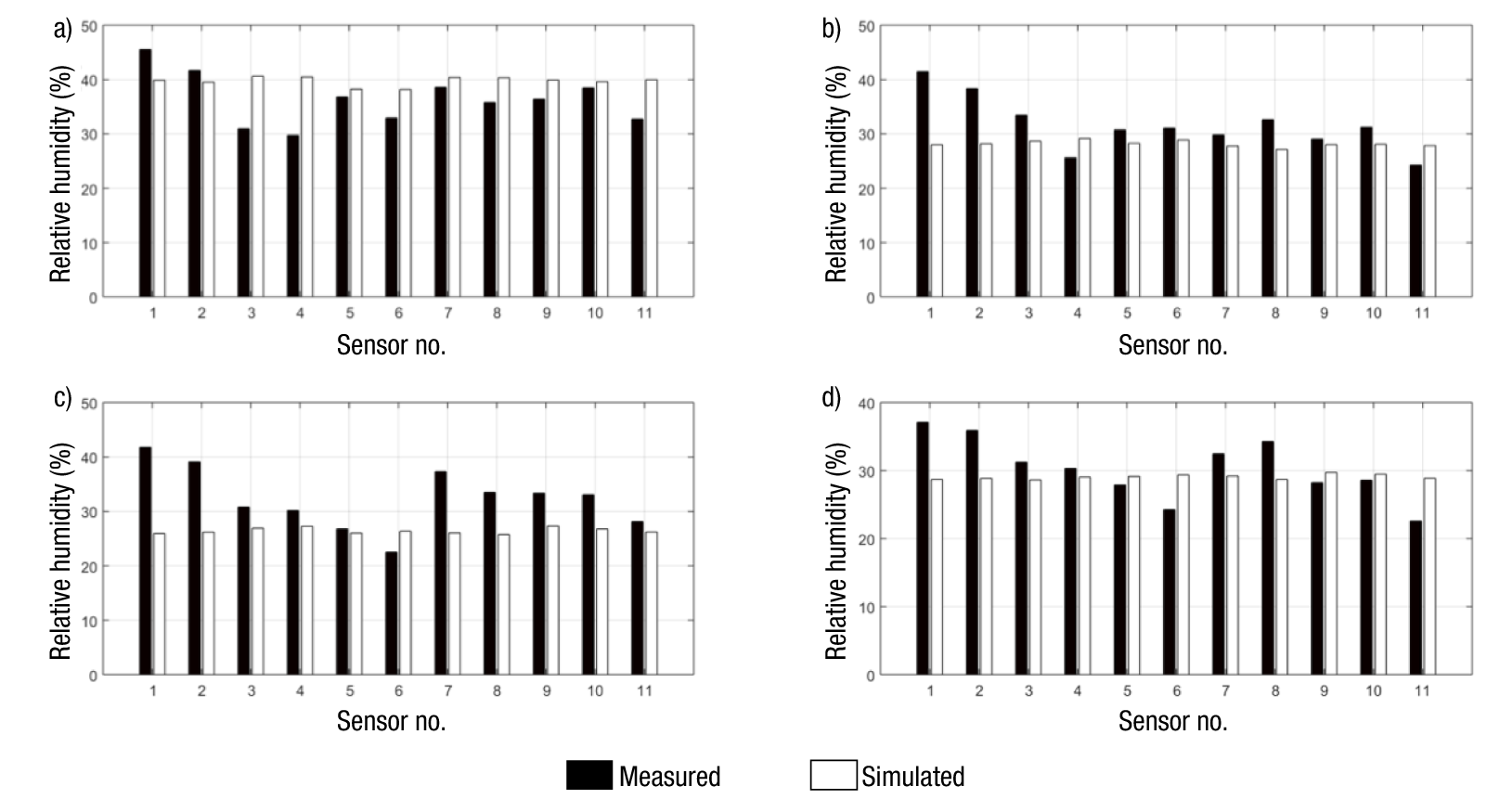
Figure 4 Comparison of measured and simulated relative humidity at 11 sensors located in the experimental greenhouse. Dates: a) 03/20/2014, b) 03/21/2014, c) 03/22/2014 and d) 03/25/2014.
The highest air humidity concentration was observed in the growing zone (0.0132 kgH2O·kgair -1); this occurs mainly due to the transpiration phenomenon. Furthermore, higher humidity was concentrated in the area close to the operating hydrophanes and where there was lower air flow velocity (0.0141 kgH2O·kgair -1), which is usually in the center and opposite to the air inlet. Regarding the above, it can be stated that there is a directly proportional relationship of humidity concentration and air velocity. Figure 5 shows the distribution of water particles dispersed by humidifiers. The 3D CFD model shows that the use of humidifiers improves humidity homogeneity inside the greenhouse (Figure 5D).
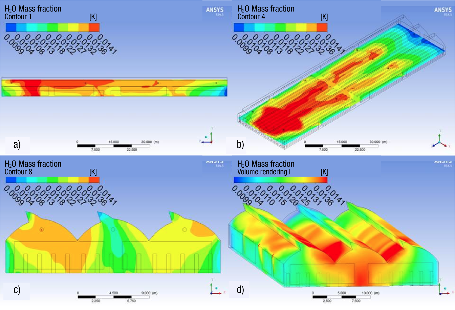
Figure 5 Air humidity distribution inside the greenhouse on March 20, 2014: a) side view in the central part of the greenhouse, b) top view at 2 m height from the ground, c) front view in the center of the greenhouse and d) 3D view of air humidity.
The 3D CFD model developed and compared with experimental measurements had an adequate adjustment with an overall average error of 0.11 to 3.43 °C and 0.44 to 10.80 % for temperature and air humidity, respectively. Making use of a fogging system on the hottest days of the year (March-June) can reduce temperature and increase humidity inside the greenhouse.
Conclusions
The 3D CFD model developed allowed to visualize the distribution of air temperature and humidity graphically and numerically inside the naturally ventilated greenhouse equipped with humidifiers. The model allows observing that the use of humidifiers improves the homogeneity of air temperature and humidity, mainly when low wind speeds are identified. This was attributed to the humidifiers, and not to the wind speed, because there were no high wind speeds inside the greenhouse. Future studies could implement the model in greenhouses with different crops and structural conformations.

