


 text in
  English (pdf)
 Article in xml format
 Article references
 Send this article by e-mail
 Cited by SciELO
  Similars in
SciELO
Similars in
SciELO 
 Permalink
Introduction
The changes that man makes to channels, which in turn modify their natural condition of equilibrium, can be beneficial or harmful to the operation and behavior of the river. Moreover, the same action can be beneficial in one river and harmful in another (Comisión Nacional del Agua [CONAGUA], 2013b). Floods are among the phenomena that can cause changes in runoff.
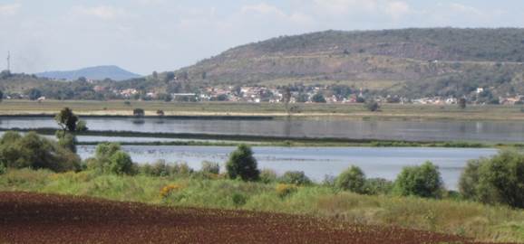
In Mexico, there is a traditional irrigation system called entarquinamiento (spate irrigation), which falls into the flood irrigation category, also known as cajas de agua (water boxes), which can be defined as variable extensions of land surrounded by embankments that are intended to store water, moisten the soil, and serve as a crop area (Palerm-Viqueira & Martínez-Saldaña, 2000; Sánchez-Rodríguez, 2005). Spate irrigation basically consists of diverting a natural water flow to plots surrounded by an embankment approximately 1.5 m high (Figure 1). According to Mollard and Walter (2008), this is a millenary technique based on the controlled flooding of a plot surrounded by a dike. The box dimensions, according to Palerm-Viqueira (2002), range from 5 to 100 ha, although in some cases they can reach 0.25 ha, which are known as pantles. In northeast Africa, particularly Eritrea, similar techniques called jeriffs have been found (Tesfai & Stroosnijder, 2000).
Certain effects generated by traditional systems have been intentional, and others not entirely, including ecological conservation, in contrast to the overexploitation of the environment with modern systems (Agarwal & Narain, 1997). In this sense, flood irrigation leads to an increase in the level of shallow groundwater (Ochoa, Fernald, Guldan, & Shukla, 2007); in the specific case of spate irrigation, agrological and phytosanitary benefits have been documented in terms of improved agricultural soils, pest control, ecological remediation (López-Pacheco, 2002), aquifer recharge (Cháirez-Araiza & Palerm-Viqueira, 2008) and other unintended effects of the use of this technique. Therefore, the objective of this work was to demonstrate that spate irrigation systems generate unintended effects such as flood control, in a 100-year return period, in the presence of maximum floods.
Materials and methods
The cartography used for this research was mostly provided by the Instituto Nacional de Estadística y Geografía (National Institute of Statistics and Geography; INEGI): a digital elevation model (Mexican elevation continuum [CEM]) with a resolution of 15 m (INEGI, 2013b), a Series II edaphological map with a 1:250 000 scale (data obtained between 2002 and 2007; INEGI, 2006), a Series V land use and vegetation map with a 1:250 000 scale (INEGI, 2013a), a climatology map with a 1:1 000 000 scale (INEGI, 2008) and a hydrographic network map with a 1:50 000 scale (INEGI, 2010).
Additionally, we used a GPS (eTrex 20, Garmin®, USA), a 20-m flexometer (PRO-20ME, PRETUL®, Mexico), the Banco Nacional de Datos de Aguas Superficiales (National Surface Water Data Bank; BANDAS) (CONAGUA, 2013a), and the ERIC III (Instituto Mexicano de Tecnología del Agua [IMTA], 2009), google earth, HEC-HMS 4.2.1 (U.S. Army Corps of Engineers, 2017) and ArcGIS 10.2.2 (Environmental Systems Research Institute [ESRI], 2014) programs, the last with the HEC-GeoHMS 10.1, HEC-GeoRAS 10.1 and ArcBruTile extensions.
Study area
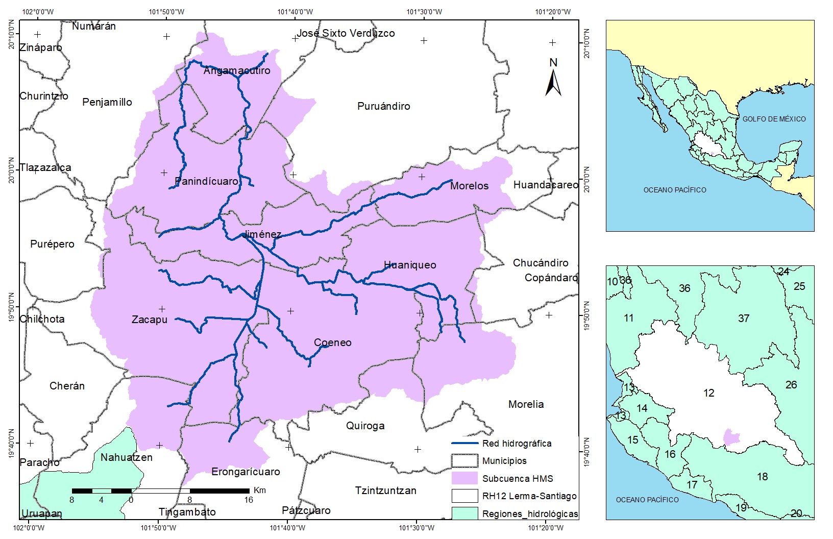
The geographical location of the spate irrigation system area is from 19° 50’ 00’’ to 19° 56’ 00’’ NL and from 101° 40’ 00” to 101° 31’ 00” WL (Figure 2), which is within the Angulo River sub-basin, which belongs to the Lerma-Chapala basin. This area is integrated into the 12 Lerma-Santiago Hydrological Region, with an area of 2 062 km2 (from 19° 35’ to 20° 15’ NL and from 101° 20’ to 102° 00’ WL) covering 15 municipalities: Angamacutiro, Chucándiro, Coeneo, Erongarícuaro, Huaniqueo, Jiménez, Morelia, Morelos, Nahuatzen, Panindícuaro, Penjamillo, Purépero, Puruándiro, Quiroga, and Zacapu (Figure 3).

Edaphology. The type of soil in the study area is mainly clay (49.50 %) and silty (47.85 %), so it can be said that not only one dominates in terms of occupied area (Table 1).
Table 1 Area occupied by soil type in study area.
| Entity | Area | |
|---|---|---|
| ha | % | |
| Silt | 98 674.81 | 47.85 |
| Clay | 102 058.60 | 49.50 |
| Water | 3 147.69 | 1.53 |
| Human settlement | 2 309.40 | 1.12 |
| Total | 206 190.51 | 100.00 |
Source: Instituto Nacional de Estadística y Geografía (INEGI). (2006). Carta edafológica Serie II. Retrieved from http://www.inegi.org.mx/geo/contenidos/recnat/edafologia/default.aspx
Land use and vegetation. Figure 4 shows that almost half the land in the study area is for agricultural-livestock-forestry use (44.68 %), while hydrophilic halophyte vegetation occupies the smallest area (0.01 %) (Table 2).
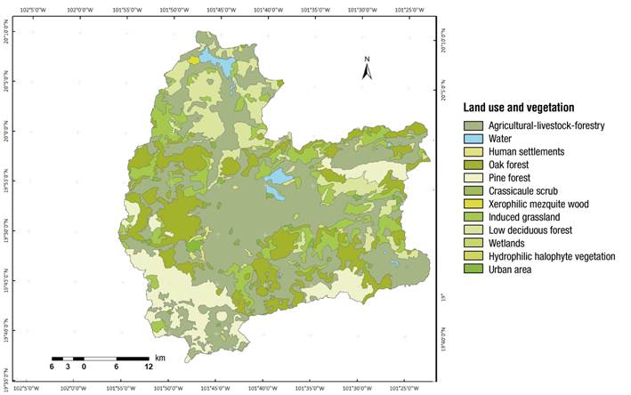
Table 2 Land use and vegetation area in the study area.
| Land use and vegetation | Area | |
|---|---|---|
| ha | % | |
| Human settlements | 2 021.25 | 0.98 |
| Pine forest | 24 430.52 | 11.85 |
| Oak forest | 35 357.15 | 17.15 |
| Waterbodies | 2 955.49 | 1.43 |
| Agricultural-livestock-forestry | 92 107.41 | 44.68 |
| Induced grassland | 24 822.18 | 12.04 |
| Hydrophilic halophyte vegetation | 17.71 | 0.01 |
| Low deciduous forest | 20 889.21 | 10.13 |
| Wetlands | 240.24 | 0.12 |
| Urban area | 2 371.54 | 1.15 |
| Crassicaule scrub | 650.52 | 0.32 |
| Xerophilic mezquites | 265.68 | 0.13 |
| Total | 206 128.90 | 100.00 |
Source: Instituto Nacional de Estadística y Geografía (INEGI). (2013a). Uso de suelo y vegetación, Serie V. Retrieved from https://www.inegi.org.mx/temas/mapas/usosuelo/
Tributary area of each channel
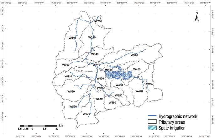
Determination of the areas of influence of each channel, within the study area, was made by means of the topography provided by the CEM, and was defined based on the characteristic slopes of each area by means of the HEC-GeoHMS program. This was done because they are tributary areas or surfaces that provide runoff to the channel (Figure 5).
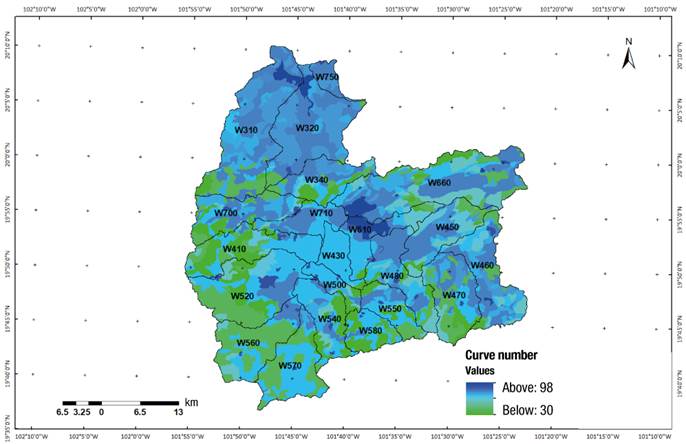
Runoff curve number
The runoff curve number (CN) method for estimating runoff depth is based on CN-tabulated (dimensionless) values, which were developed by the Soil Conservation Service (SCS) of the United States, where the curve number chosen will depend, in practical terms, on the soil texture (hydrologic soil group) and land use, the density of plant cover (hydrologic condition) and the possible existence of soil conservation practices (Pérez-Nieto, Ibáñez-Castillo, Arellano-Monterrosas, Fernández-Reynoso, & Chávez-Morales, 2015). In Mexico, this method is used due to its simplicity and lack of instrumentation in the basins (Alonso-Sánchez, Ibáñez-Castillo, Arteaga-Ramírez, & Vázquez-Peña, 2014).
In this study, the CN value was obtained from data tabulated by Mockus et al. (2009), based on soil type and land use (Table 3), in combination with the edaphological map (Domínguez-Mora et al., 2008). The spatial distribution, according to the NC obtained, is shown in Figure 6.
Table 3 Runoff curve number.
| Description | Hydrologic group | |||
|---|---|---|---|---|
| A | B | C | D | |
| Agricultural-livestock-forestry | 62 | 71 | 78 | 81 |
| Human settlement | 39 | 61 | 74 | 80 |
| Coniferous forest | 25 | 55 | 70 | 77 |
| Oak forest | 36 | 60 | 73 | 79 |
| Waterbody | 100 | 100 | 100 | 100 |
| Scrub | 34 | 58 | 71 | 78 |
| Mezquites | 68 | 79 | 86 | 92 |
| Grassland | 39 | 61 | 74 | 80 |
| Tropical dry forest | 45 | 66 | 77 | 83 |
| Wetlands | 68 | 79 | 86 | 92 |
| Halophyte vegetation | 68 | 79 | 100 | 100 |
| Urban área | 77 | 85 | 90 | 92 |
Source: Mockus, V., Werner, J., Woodward, D. E., Nielsen, R., Dobos, R., Hjelmfelt, A., & Hoeft, C. C. (2009). Hydrologic soil groups. United States of America: NRCS.
Subsequently, the CNs obtained were adjusted, since the SCS defines three soil moisture conditions: I-dry (wilting point), II-medium moisture and III-completely wet (field capacity). The CNs for soil conditions I and III were calculated with the equations proposed by Neitsch, Arnold, Kiniry, and Williams (2011).
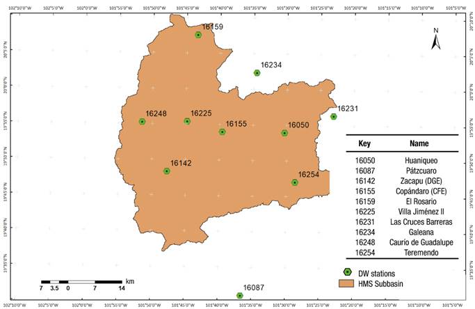
Weather stations
The weather data used in the model were from 1983 to 2012 (30 years), which were obtained from Sistema Meteorológico Nacional (National Meteorological System) stations operated by Comisión Nacional del Agua (National Water Commission), located both inside and outside the study area (Figure 7).
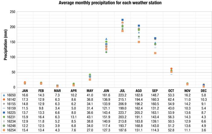
Precipitation
The behavior of the average monthly precipitation recorded at the weather stations closest to the study area is shown in Figure 8.
Missing precipitatin data were calculated by the inverse square distance method (Equations 1 and 2) (Gallegos-Cedillo, Arteaga-Ramírez, Vázquez-Peña, & Juárez-Méndez, 2015).
Where P x is the missing precipitation data (mm), P i is the precipitation recorded at the surrounding auxiliary stations (minimum two) at the date of the missing data (mm) and D i is the distance between each surrounding station and the incomplete station (km).
Calculation of maximum expected rainfall
To calculate the maximum rains in different return periods, namely 10, 20, 50 and 100 years, we used the methodology proposed by the SCS, which consists of obtaining and grouping the maximum rains presented in a certain recording period (30 years in this case), calculating statistical parameters of the theoretical distribution and adjusting the rains.
Frequency analysis
The objective of hydrological information frequency analysis is to relate the magnitude of events, especially extreme ones, to their occurrence through the use of probability distributions, for which it is assumed that the hydrological information analyzed is independent of space and time (Chow, Maidment, & Mays, 1988). In this case, frequency analysis of extreme rains was carried out by the by the method of moments, for which the original rainfall values were fitted to a theoretical distribution: normal, log normal, pearson III (gamma), log pearson and Gumbel.
Kolmogorov-Smirnov goodness-of-fit test
To verify whether the data fittted the proposed methodology, the Kolmogorov-Smirnov goodness-of-fit test was applied (Equation 3), which consists of comparing the observed probability distribution function [F 0 (X m )] (Equation 4) with the theoretical one [F(X m )]:
where m is the order number of the given value, X m is a list from lowest to highest and n is the total number of data.
To use this test, the proposed null hypothesis (H0) is that the probability distribution function is D (α, β).
The maximum observed difference (D) is compared with a Kolmogorov-Smirnov table statistic; if D is lower, the theoretical distribution is accepted. The value of this statistic depends on the length of the record and the level of significance. If several distributions are accepted, the one with the smallest observed difference is chosen.
Rainfall-runoff relationship
According to Aparicio-Mijares (2001), precipitation records are more abundant than runoff records, and do not change due to anthropogenic modifications in the basin; therefore, it is recommended to use methods that determine runoff from rainfall data and basin characteristics. The CN method, for the calculation of precipitated depth to runoff depth, was developed in 1950 by the U.S. Department of Agriculture. The main parameters involved in the process of converting rainfall to runoff are the area of the basin, the amount of rainfall, the slope of the basin, the time of concentration, the vegetation, and the spatial and temporal distribution of the rain.
For the above, Equations 5 and 6 are used, which estimate the direct runoff from a storm (Chow et al., 1988):
for P > 0.2 S, otherwise Pe = 0
where Pe is the direct runoff depth (mm), P is the precipitation (mm), S is the maximum potential retention (mm).
The most commonly used methodological tool to model the rainfall-runoff process is based on the unit hydrograph theory (Juárez-Méndez, Ibáñez-Castillo, Pérez-Nieto, & Arellano-Monterrosas, 2009), which assumes that the discharge at any time is proportional to the volume of runoff evenly distributed in the basin (Snider et al., 2007), as it considers the rainfall depth, the area, shape, slope and vegetation of the basin, although not explicitly (Aparicio-Mijares, 2001). The fundamental principles of base flow time constant, overlap and proportionality make the unit hydrograph an extremely flexible tool for developing synthetic hydrographs.
Chow et al. (1988) mention that the dimensionless SCS hydrograph is a synthetic triangular unit hydrograph transformed into a curvilinear shape, in which the flow rate is expressed by the ratio of the flow rate (q) with respect to the peak flow rate (q p , m3·s-1·mm-1) and the occurrence time of the peak in the unit hydrograph (T p , h). If a unit hydrograph of 1 mm is considered, it can be demonstrated that:
where A is the drainage area (km2) and T p is egual to 1.67 h d according to the SCS.
Additionally, Aparicio-Mijares (2001), in SCS basins, indicates that in the unit hydrographs the delay time (t r ) is egual to 0.6 T c , where T c is the time of concentration of the basin. The T p can be expressed in terms of the t r and the duration of the effective rainfall d e (Equation 8):
On the other hand, runoff can be estimated in two ways: 1) probabilistic prediction and 2) "real time" forecast, so it is necessary to adequately characterize the runoff and the phenomena related to it (the rain and the basin). In addition, based on the laws of physics and probability theory, a series of models needs to be developed, which should be manageable in practice, and lead to correct forecasts and predictions (Domínguez-Mora, 1990).
Once the runoff comes down from the slopes, it begins its route in the channels that are already defined. The channels cushion the speed and temporarily store part of the flow. Therefore, at the end of the channel, an outlet hydrograph different from the initial one is generated.
There are different methods for calculating flood routing in channels; one of the simplest is the method described by Muskingum (Equation 9) (Aparicio-Mijares, 2001):
where I i and O i are the ordinates of the inlet and outlet hydrographs (m3·s-1), respectively; the coefficients C1, C2 are C3 are calculated as follows:
where C 1 + C 2 + C 3 = 1, K and x are the Muskingum parameters, the first in time units and the second dimensionless.
The spate irrigation system as a storage area
The spate irrigation system formed by "boxes" works similar to a storage dam, but without discharging immediately. It is considered that in times of major floods, runoff can be divided between a maximum volume stored by the boxes and the continuation of its course in the channel.
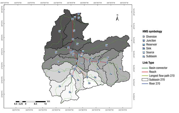
HEC-HMS model
According to McCuen (1998), hydrological models are simplified representations of real hydrological systems that allow studying the functionality and response of a basin to several input conditions, to better understand hydrological events. The Hydrologic Engineering Center-Hydrologic Modeling System (HEC-HMS) is a model of hydrologic parameters aggregated by sub-basin, with the option of a model distributed in space; it subdivides a basin into sub-basins, taking as the initial criterion the tributaries of the main current (Miranda-Aragón, Ibáñez-Castillo, Valdéz-Lazalde, & Hernández-de la Rosa, 2009). In the present work, this model was used, since it simulates the precipitation and runoff processes of the dendritic basin systems. In addition, it is applied in diverse geographical areas to solve a large number of problems; this includes the water supply to the watershed and flood hydrology. In Mexico, runoff from urban or natural basins is studied per extreme weather event (Vargas-Castañeda, Ibáñez-Castillo, & Arteaga-Ramírez, 2015).
Hydrographs, or some of their elements (such as peak flow), are used in the planning and design of water control structures, as well as to show existing hydrological effects or proposed changes in land use (Snider et al., 2007). Hydrographs produced by the HEC-HMS are used directly or together with other software to study water availability, urban drainage, flow forecasting, future urbanization impact, reservoir spillway design, flood damage reduction, floodplain regulation, and systems operation (U.S. Army Corps of Engineers, 2016). On the contrary, hydrological studies with traditional techniques for surface runoff do not present the study needs for small structures.
Results and discussion
Figure 9 shows the elements of the model made by means of HEC-GeoHMS to evaluate the functioning of the "embankments" in the basin.
The delay time, which is related to the runoff curve number (corrected for slope), the slope of the input area, the hydraulic length of the channel and the area, for the tributary zone that makes up the basin, are presented in Table 5.
Table 5 Characteristics of the basin’s input areas.
| Identification number | Name | Slope (%) | Ruoff curve number | Delay time (h) | Area (km2) |
|---|---|---|---|---|---|
| 1 | W310 | 9.97 | 89.90 | 4.11 | 209.25 |
| 2 | W320 | 8.88 | 92.32 | 2.67 | 167.71 |
| 3 | W340 | 16.36 | 85.63 | 1.69 | 77.98 |
| 4 | W410 | 14.59 | 76.97 | 4.74 | 108.04 |
| 5 | W430 | 5.27 | 87.55 | 2.23 | 40.30 |
| 6 | W450* | 14.51 | 87.69 | 1.98 | 90.09 |
| 7 | W460* | 14.56 | 89.57 | 2.29 | 113.51 |
| 8 | W470* | 21.22 | 83.16 | 2.27 | 102.46 |
| 9 | W480* | 13.81 | 86.55 | 2.25 | 92.80 |
| 10 | W500 | 6.06 | 86.01 | 2.38 | 31.42 |
| 11 | W520 | 14.42 | 80.30 | 3.28 | 160.42 |
| 12 | W540 | 9.51 | 84.39 | 2.82 | 79.67 |
| 13 | W550 | 14.68 | 83.15 | 1.95 | 55.33 |
| 14 | W560 | 18.86 | 79.27 | 2.50 | 109.22 |
| 15 | W570 | 15.23 | 81.91 | 2.76 | 104.28 |
| 16 | W580 | 14.61 | 78.22 | 1.74 | 50.32 |
| 17 | W610* | 7.98 | 88.77 | 2.66 | 68.23 |
| 18 | W660 | 13.15 | 87.62 | 3.50 | 231.15 |
| 19 | W700 | 14.82 | 85.49 | 2.18 | 94.11 |
| 20 | W710 | 10.18 | 90.78 | 1.44 | 53.82 |
| 21 | W750 | 7.73 | 93.19 | 1.44 | 21.20 |
| Total 2 062.00 | |||||
*Areas that affect the outlet of the spate irrigation system.
On the other hand, Table 6 presents the 33 sections of the channel and the K parameter for the application of the Muskingum method. This parameter was obtained by taking as the average speed the peak of 2.5 m·s-1, whereas x was proposed as 0.2 (since x is close to 0 in channels with a small slope and a high flow, and a value of 0.5 is for large slopes).
Table 6 Muskingum K parameter and length of the basin’s channel sections.
| Identification number | Name | Length (m) | K (h) |
|---|---|---|---|
| 1 | R20 | 16845.48 | 1.25 |
| 2 | R30 | 3101.20 | 0.23 |
| 3 | R40 | 34711.09 | 2.57 |
| 4 | R50 | 8015.28 | 0.59 |
| 5 | R60 | 9997.37 | 0.74 |
| 6 | R80 | 5354.49 | 0.40 |
| 7 | R100 | 8080.36 | 0.60 |
| 8 | R110* | 8987.70 | 0.67 |
| 9 | R120 | 6020.07 | 0.45 |
| 10 | R140* | 6091.56 | 0.45 |
| 11 | R150 | 22456.40 | 1.66 |
| 12 | R160 | 3593.74 | 0.27 |
| 13 | R170 | 9358.08 | 0.69 |
| 14 | R180 | 2279.04 | 0.17 |
| 15 | R190 | 734.57 | 0.05 |
| 16 | R200 | 10219.93 | 0.76 |
| 17 | R210 | 13559.46 | 1.00 |
| 18 | R220 | 16085.61 | 1.19 |
| 19 | R230 | 4864.91 | 0.36 |
| 20 | R240 | 5081.50 | 0.38 |
| 21 | R250 | 3642.07 | 0.27 |
| 22 | R260 | 12736.06 | 0.94 |
| 23 | R270 | 1351.88 | 0.10 |
| 24 | R280 | 14508.25 | 1.07 |
| 25 | R290 | 14310.58 | 1.06 |
| 26 | R130* | 2127.76 | 0.16 |
| 27 | R630* | 7947.59 | 0.59 |
| 28 | R90 | 4404.01 | 0.33 |
| 29 | R680 | 28531.42 | 2.11 |
| 30 | R720 | 1601.10 | 0.12 |
| 31 | R70 | 4296.14 | 0.32 |
| 32 | R770 | 2063.31 | 0.15 |
| 33 | R10 | 4721.27 | 0.35 |
*Channel sections that affect the runoff at the outlet of the spate irrigation system.
These previous results are the inputs with which the program executes a series of procedures in order to obtain the final results.
The models made with HEC-HMS, where the outlet hydrograph is obtained in each of the parts of interest, are shown in Figure 10, and the unintended effect of the use of spate irrigation can be observed. In addition, the figure shows that for a design storm with a 100-year return period, the peak flow is 535.5 m3·s-1 and the peak discharge is 0 m3·s-1, which reflects an operation similar to that of a storage dam. It should be borne in mind that water boxes do not fully trap rainwater, as a portion is held in the channel by subsurface runoff, especially when the rainy season has already begun and there are severe storms.
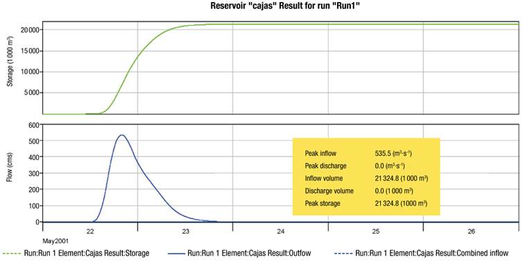
Figure 10 Hydrograph at the outlet of the spate irrigation system for a 100-year return period (167.8 mm of rainfall).
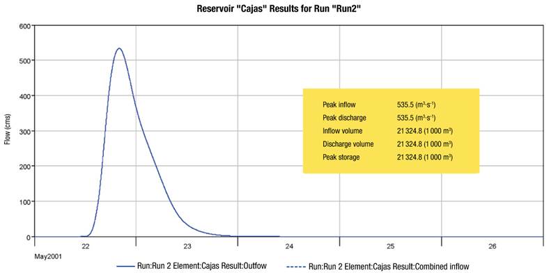
In the case of the non-spate irrigation system (Figure 11), the water that feeds the box system is not diverted to it, but rather the flood flow is kept flowing in the main channel. This model shows the existence of a considerable flow (535.5 m3·s-1) at the system outlet; that is, if the spate irrigation system is suppressed, some localities located in the study area could be affected by floods.
Conclusions
This research conducted on the Coeneo-Huaniqueo Valley embankment system (5 337.82 ha) proves the benefit of using spate irrigation in this area, since it is considered a hydraulic buffer zone that serves as a flood mitigation measure in the downstream area. If this technique were to be suppressed in the region, another way of controlling floods would have to be considered. Therefore, beyond taking deliberate actions aimed at diminishing, and even eliminating, the spate irrigation technique, measures would have to be taken based on science and technique to find a balance between the medium- and long-term benefits.
Based on the above, the evidence gathered during this research, from the hydrological and hydraulic point of view for the spate irrigation system, suggests that the technique in question generates unintended effects such as flood control in human settlements and prevention of severe crop losses due to flooding, among others.
The spate irrigation system, like other traditional systems for water use and management, is located in an atmosphere unfavorable for its conservation and preservation, because it is considered an obsolete practice that wastes water, among other arguments. Therefore, it is of great importance to provide elements that show its intended and unintended effects, this with the support of specialists in ecology, agrology, agronomy and hydrology.

