


 text in
  English (pdf)
 Article in xml format
 Article references
 Send this article by e-mail
 Cited by SciELO
  Similars in
SciELO
Similars in
SciELO 
 Permalink
Introduction
The expansion of protected agriculture has led to an increase in crop yields. To a great extent, this increase has been made possible by the capacity achieved in the management of climate variables, which allows optimal crop performance. Achieving this expansion implied the technological adaptation of the system, originally conceived under characteristics restrictive to practically any climatic condition. However, despite the achievements, technological constraints still persist in the implementation of this production system. The current situation requires a personalized management approach that deals with the interaction of the biosystem (physical-biological-environmental) (Boulard, Roy, Pouillard, Fatnassi, & Grisey, 2017; García-Martínez, Balasch, Alcon, & Fernández-Zamudio, 2010; Maher, Sami, & Hana, 2018; Piscia et al., 2012).
In Mexico, the area devoted to crop production in protected and semi-protected systems exceeds 30,000 ha, and continues to grow; however, due to the country’s climatic diversity, it is still considered a risky activity due to environmental management issues, owing to the use of medium and low technology greenhouses (Servicio de Información Agroalimentaria y Pesquera [SIAP], 2013). Despite these circumstances, the agricultural sector has been able to maintain crop production, thereby guaranteeing food to a logarithmically growing population (Moreno-Reséndez, Aguilar-Durón, & Luévano-González, 2011). The challenges are to make Mexican producers more competitive by transferring technology and to sustain it by increasing the protected agriculture area (Avendaño-Ruiz & Schwentesius-Rindermann, 2005).
The ability to manipulate environmental conditions within a greenhouse allows for production control, increased productivity and quality, and an extended growing period, which is not possible through traditional production systems (Hanan, 1998; van Straten & van Henten, 2010). However, greenhouse upgrading is dependent on climatic variations and the investment capacity of producers to acquire and use heating systems, air extractors, and automated irrigation and fertilization systems (Juárez-López et al., 2011). In addition, greenhouse production systems should be optimized, for which the presence of multiple factors in climate response and the inclusion of economic models must be taken into account (Hasselmann & Hasselmann, 1998).
A biological system transfers heat and mass, and within a greenhouse there are sources consuming heat, pollutants and water vapor (Rico-García, Castañeda-Mirada, García-Escalante, Lara-Herrera, & Herrera-Ruiz, 2007). In this sense, microclimate modeling has evolved with the use of subroutines or models that consider the biological system. According to Norton, Sun, Grant, Fallon, and Dodd (2007), these subroutines allow the modeling of plant transpiration, the production or consumption of CO2 and the programming of boundary conditions. Flores-Velázquez and Villarreal-Guerrero (2015) mention that a routine for this type of modeling is, firstly, the calculation of the biosystem’s inside temperature based on net solar energy, and secondly, the division of solar energy into convective and latent flows based on local conditions. The latter depends on heating and water vapor exchanges (stomata and aerodynamics) between the matrix of the porous medium and the air inside each mesh of the aboveground part of the crop (represented by a porous medium).
The aforementioned models allow obtaining more real and detailed results based on the biological response of the crops, for which it is necessary to consider their physical aspects, the use of climate control equipment in the greenhouse (Ito & Hattori, 2012; Montero et al., 2013; Piscia et al., 2012), the interaction of the climate considering the effect of evotranspiration (Bouhoun-Ali, Bournet, Danjou, Morille, & Migeon, 2014; Farber, Farber, Grabel, Krick, & Uberholz, 2017; Tamimi & Kacira, 2013), photosynthesis (Boulard et al., 2017; Roy, Pouillard, Boulard, Fatnassi, & Grisey, 2014) and stoma resistance (Bouhoun-Ali, Bournet, Cannavo, & Chantoiseau, 2017).
Over the past 20 years since its creation, a tool based on numerical methods for greenhouse climate management, known as computational fluid dynamics (CFD), has been constantly improved. This tool has brought significant results applicable to the development of the protected agriculture sector (Flores-Velázquez, Mejía-Saenz, Montero-Camacho, & Rojano, 2011; Norton et al., 2007).
One of the main problems facing passive greenhouse crop production is excess heat, which accumulates at specific times of the year and day. This implies that the accumulated radiation in the thermal infrared wavelength must be evacuated to optimize energy consumption (Shen, Wei, & Xu, 2018) and water consumption (Katsoulas, Sapounas, de Zwart, Dieleman, & Stanghellini, 2015). In this type of greenhouse, natural ventilation systems are used (opening and closing windows) to prevent the temperature from rising; however, it is possible that at times of maximum radiation it may be necessary to use an auxiliary ventilation system alone (Chia-Ren, Ting-Wei, Ren-Kai, Tso-Ren, & Chih-Kai, 2017; Flores-Velázquez &Villarreal, 2015) or combined (Flores-Velázquez, Montero, Baeza, & López, 2014).
There is a trend towards using agricultural production systems such as the greenhouse, plant factory and vertical farm, among others (Al-Kodmany, 2018; de Anda & Shear, 2017), in urban areas, so it is considered necessary to quantify the cost of the non-subsidized domestic electricity tariff. This cost is estimated based on the operating time of the fans, which would be when the outside temperature exceeds 30 °C. Derived from this analysis, the results are extrapolated with data from local weather stations to analyze the operating cost of the fans by municipality.
Therefore, the objective of this work was to model the environment of a zenith greenhouse cultivated with tomato by means of CFD, to propose environmental management alternatives and to estimate the energy expenditure for the use of fans and the economic cost thereof with two commercial tariffs (domestic and agricultural).
Materials and methods
The greenhouse used for microclimate analysis and validation is located in the municipality of Soledad de Graciano Sánchez, San Luis Potosí, Mexico, with coordinates 22° 13’ 50’’ N and 100° 51’ 35’’ W, at 1 835 masl. The greenhouse structure has an approximate area of 1,000 m2 (Table 1), a translucent polyethylene cover and retractable curtains on each side, as well as in each overhead window.
Table 1 Geometricdimensions of the computational model.
| Greenhouse dimensions (m) | Outside domain dimensions (m) | Crop area dimensions (m) |
|---|---|---|
| 34 x 32 x 4.75 | 170 x 192 x 22.35 | 31 x 30 x 0.7 |
The greenhouse was equipped with six probes (Vaisala HMP50, Campbell Scientific®, USA), of which five recorded the temperature and relative humidity inside the greenhouse (probes 1, 2, 3, 5 and 6). The wind speed and direction/solar radiation probe (probe 4) was placed on the ridge (outside the greenhouse), at 8 m high. This last one recorded the temperature and relative humidity outside the greenhouse. Of the probes placed inside the greenhouse, three were located in the center of each span. Probe 1 was placed in the span near the control cabin, probe 2 in the central span, and probe 3 in the opposite span (Figure 1).
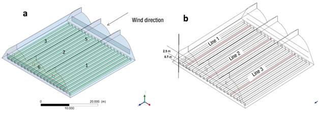
Figure 1 a) Simulated greenhouse model and location of sensors and b) longitudinal profiles in the center of each span and plan view at two heights (0.7 and 2.5 m).
Inside the greenhouse, ball-type red tomato (Lycopersicum esculentum) was cultivated, sown in a quincunx arrangement with a density of 4.4 plants·m-2. Plants were distributed in 60-cm ridges, giving a total of 20 beds (seven beds in two of the spans and six in the other one), 1.8 m of corridor (from half bed to half bed, from the irrigation system strip) and 1.2 m of free space between ridges.
To validate the model, the environmental readings obtained from the instruments installed in the greenhouse were used. These readings were recorded and stored from 6:16 am on June 21, 2014 until 2:52 pm on July 19 of the same year. The data recorded were: temperature, relative humidity, wind speed and radiation, both inside and outside the greenhouse. The stored information was downloaded and then processed in Excel, Microsoft®, where a focus was made at two time intervals: from 12:30 pm to 2:30 pm as the warm period of the day, and from 4:30 am to 5:30 am as the cold period. The total averages of the variables recorded in each probe were obtained and then used to determine the model’s initial conditions.
ANSYS® Fluent® software was used for the development and numerical simulation of the CFD model. As a previous phase, the geometry and mesh of the model were generated in which the boundary conditions were defined; for this purpose, the ventilation analysis was performed in three dimensions. The geometry, domain and mesh of the model were developed in ANSYS® Workbench, with Design Modeler and Meshing tools. Within the process, solution is given to the transport equations, which were discretized in algebraic equations and calculated by numerical methods.
The greenhouse was simulated by CFD, as well as the natural ventilation system, from which the inlet and outlet airflows are quantified. The inlet speed, as a boundary or starting condition, was established according to the wind speed values measured with the sensors installed. The space occupied by the crop was simulated and assigned porous medium properties.
Additionally, hypotheses were established regarding the configuration of the simulation, for which the conditions of the model and of the variables involved to obtain the solution were considered (Table 2).
Table 2 Simulation hypothesis, contour characteristics and physical properties used as parameters in the model solution.
| Parameters | Hypothesis |
|---|---|
| Physical properties | |
| Solution | Segregated |
| 3D simulation | |
| Implicit formulation | |
| Absolute speed | |
| Time condition | Steady-state analysis (second order) |
| Viscosity model | Standard k-ε (two equations) |
| Activated flotation effect | |
| Standard wall treatment | |
| Energy equation | Activated |
| Pore formulation | Surface speed |
| Gradient option | Cell-based |
| Contour characteristics | |
| Inlet domain | Inlet speed: constant |
| Momentum: orthogonal to the boundary | |
| Turbulence, intensity and increase in viscosity | |
| Outlet domain | Outlet pressure: constant |
| Zero pressure and same turbulence condition | |
| Wind speed | Profile: constant (m·s-1) |
| Porous medium treatment | Mesh: Porous jump |
| Crop: Porous zone | |
| Heat source | Constant from the ground: Boussinesq’s hypothesis |
| Flotation effect on the activated turbulence model | |
The simulated scenarios consisted of a natural ventilation system in which the behavior of temperature, wind speed and its effect on the ventilation rate in the environment generated inside the greenhouse were described. In addition, an alternative for the management of high temperatures with natural ventilation in combination with mechanical ventilation was proposed and described (Table 3), and its use was evaluated based on the cost and time of operation in the day.
Table 3 Model simulation scenario: natural ventilation.
| Variable | Natural ventilation | Combined ventilation |
|---|---|---|
| Outside temperature (K) | 295.7 (warm) 288.04 (cold) | Constant 295.7 |
| Outside wind speed (m·s-1) | 2.41 (warm) 1.67 (cold) | Constant 2.41 |
| Heat source (W·m-2) | 200 (constant from the ground) | 200 (constant from the ground) |
| Outlet pressure | Normal at boundary | (FAN) Constant 10 Pa |
Statistical evaluation of the computational model
For the evaluation of the model, an analysis of variance was carried out with the data obtained experimentally and with the data simulated in Fluent®. The comparison was made for the two periods (warm and cold) in a natural ventilation scenario, where temperature (°C) and wind speed (m·s-1) were considered as main factors. Additionally, based on the position of the sensors inside the greenhouse, longitudinal profiles were made in the center of each span.
For statistical analysis, point data of the climate variables of the sensors
(discrete) and those estimated by means of simulation (continuous) were used;
these values showed normal (unbiased) behavior. Under these criteria, it was
considered appropriate to use the S
2
p estimator (Equation
1) to statistically conclude the model’s evaluation in both periods.
This gives the advantage of being able to relate the parameters of the
experimental (X) and simulated data (Y), as
well as their means (
Where:
and
The S 2 p estimator was used because it is a weighted average of the two sampling variances (Sx 2 and Sy 2 ), where the weights represent the degrees of freedom. Considering the types of data (climatic) used, the suffix p indicates that the estimated variance is a weighted measure of Sx 2 and Sy 2 ; that is, they do not have the same weight in S 2 p, but the importance of each of them depends on the number of observations in the sample. With this analysis, the acceptance or not of the hypothesis tests and, consequently, of the model was evaluated. In general, this estimator is appropriate to obtain approximations of population variance in inferential data analysis (Walpole, Myers, Myers, & Ye, 2012).
The S 2 p estimator can be used to obtain a to statistic (Equation 4) and test the hypothesis of the statistical difference of the means of the experimental and simulated data (δ = μx - μy):
For both periods, the parameters described and the corresponding statistical tests were calculated, as well as confidence intervals (Equations 5 and 6).
Once the model was evaluated, the behavior of the air inside the greenhouse and the spatial distribution of the temperature gradients in the simulated scenarios were described, both on the longitudinal (sensors 2, 5 and 6) and transversal (sensors 1, 2 and 3) profiles in the planes generated inside the greenhouse at a height of 0.7 m (at crop level) and 2.5 m (at sensor level). Ventilation rates were calculated and an analysis of the wind speed and temperature profiles was performed, as a result of the simulation that considered wind speed (m·s-1) and temperature (°C) as boundary conditions, as well as aspects of crop resistance, and window position and size.
Subsequently, the environmental conditions for tomato development and factor (temperature and wind speed) management were discussed, and alternatives were proposed to improve greenhouse ventilation through natural and mechanical ventilation. The extrapolation of the results by municipality was carried out with national meteorological databases, in which, previously, a "cleaning" process was performed in order to obtain data of more than 20 years in the State of Mexico and San Luis Potosí.
Results and discussion
Model evaluation
Warm period. Consistency between experimental and simulated data was mostly observed in the middle part of the greenhouse (Table 4). On the other hand, in the area immediately adjacent to the entry wall, there is a minor correlation, which could be due to the turbulent flows that occur because of the pressure drop, a product of the porous wall. With the above, a standard deviation between 1.13 and 0.907 was obtained; in addition, a t0 of 2.127 was estimated, with t0.025 of 2.306, so the hypothesis is rejected with statistically equal means.
Table 4 Simulated and experimental data: warm period.
| Temperatures (°C) | |||
|---|---|---|---|
| Sensor | Experimental | Simulated | Error |
| 1 | 25.50 | 24.63 | 0.87 |
| 2 | 25.68 | 25.31 | 0.37 |
| 3 | 28.54 | 24.85 | 3.69 |
| 5 | 26.34 | 23.65 | 2.69 |
| 6 | 25.71 | 26.43 | -0.72 |
Cold period. Statistical analysis for the cold period showed differences in the transversal profile between the two data sets (Table 5). The 1 K temperature gradient maintains constant similarity in the transversal direction within the greenhouse when sampling. The experimental temperature values remain stable with each other, all being above 16 °C, but none greater than 17 °C, which did not occur with the simulated data ranging from 16.41 to 19.50 °C. However, the standard deviations are from 0.207 to 0.993, and the results of the analysis of variance indicate that the 95 % confidence interval (1-α) for μx - μy has limits from -0.391 to -2.483. Therefore, the limits indicate that the means do not differ statistically, hence the hypothesis is not rejected.
Description of wind speed profiles and temperature gradients
Warm period. In the longitudinal profile of Figure 2, it can be seen that when the wind speed decreases, the temperature increases. Figure 2a shows the interior of the greenhouse, where the lowest temperatures are in the area near the side inlet window, but increase when approaching the outlet side window, whereas Figure 2b shows how the highest wind speeds extend along the plastic sidewalls of the greenhouse where the temperature is lower.

Figure 2 Average longitudinal profile of simulated temperature (○) and wind speed (●). Plan view of the spatial distribution of temperatures at two heights: a) 2.5 m and b) 0.7 m. Outside temperature 295.7 K and outside wind speed 2.41 m·s-1.
In the crop area (at 0.7 m), wind speed varies in magnitude between the corridor area and the crop area; however, temperature remains constant in the transversal profile. Longitudinally, there is a reduction in the flow to the outlet side window, so that air renewal in that area makes it difficult to regulate the temperature and, as it moves away from the inlet side window, the wind loses energy and the temperature increases to 2 K, thus having temperatures around 300 K. The temperature stratification at 0.7 m is less than at 2.5 m. In general, the wind maintains a speed of the order of 0.1 to 0.3 m·s-1 at crop level, although on the sidewalls it goes from 0.4 to 0.7 m·s-1.
Cold period. The wind speed has a tendency to decrease from the sidewalls to the center of the greenhouse, where it increases its speed, but not enough to lower the temperature, having the maximum gradient in this area. The same behavior is seen in the longitudinal profile, as well as the effect that ventilation has in the decrease and regulation of the temperature. Figure 3a shows the temperature stratification, whose values increase as the wind decreases. Wind speed remains constant between 0.1 and 0.4 m·s-1 in much of the greenhouse, but tends to zero as it approaches the outlet side window (Figure 3b).

Figure 3 Average longitudinal profile of simulated temperature (○) and wind speed (●). Plan view of the spatial distribution of temperatures at two heights: a) 2.5 m and b) 0.7 m. Outside temperature 288.04 K and outside wind speed 1.67 m∙s-1.
In the crop area, the temperature distribution is dispersed, with thermal gradients from 1 to 3 K when approaching the left sidewall. This is consistent with the maximum temperature period, indicating that the convective effect predominates over the radioactive one. This allows formulating hypotheses for climate management, in which case it is better to move the greenhouse air by pressure than by convection.
It has been observed that wind speed tends to decrease in the center of the greenhouse due to the resistance generated by the leaf area to the passage of air; in this case, the overhead window plays the role of "motorizing" ventilation. For the purposes of these simulations, from the point of view of ventilation, the crop functions as a porous medium where the movement of air decreases. Even with the highest flows obtained with the side windows open, the speed reduction puts into perspective the resistance of the crop in the ventilation process.
Calculation of ventilation rates
In Table 6, the sign represents the direction of the flow. A negative sign implies that the air enters the greenhouse, and a positive sign is the exit of the air, this for the simulation of the fluids.
Table 6 Ventilation rates estimated with CFD: warm period.
| Boundary | Position | Cold period | Warm period | |||||
|---|---|---|---|---|---|---|---|---|
| Flow
(kg·s-1) |
Flow rate
(m3·h-1) |
N Rate
(h-1) |
Flow
(kg·s-1) |
Flow rate
(m3·h-1) |
N Rate (h-1) |
|||
| Porous jump | Overhead windows | 42.993 | 126 450.0 | 24.30 | 54.74 | 160 886.2 | 30.91 | |
| Outlet side window | -1.841 | -5 414.7 | -1.05 | 6.32 | 18 596.6 | 3.57 | ||
| Inlet side window | -41.151 | -121 032.4 | -23.25 | -61.07 | -179 485.7 | -34.48 | ||
| Mass balance | 0.0 | 0.0 | 0.0 | 0.0 | 0.0 | 0.0 | ||
Based on the numerical results, it is possible to determine that opening the windows does not mean ventilating. On the one hand, it is important to capture as much air as possible, but windows are also needed to expel it, and thus favor the ventilation rate.
Under greenhouse operating conditions, simulated data show a ventilation rate of 34.48 hourly volumes; although it is low, according to what is recommended by ASHRAE (2016), it is considered a suitable growing environment.
High temperature management alternative: combined ventilation
In order to evaluate the feasibility of using mechanical ventilation as an emergent alternative in specific time periods, i.e., when external radiation increases the temperature inside the greenhouse, three motors were attached to the model, one in each span (Figure 1) at 2.5 m high. The catalogue dimensions are 1 x 1 m, which correspond to the Exafan® EX 36"-0.5 air extraction system model (Spain).
The analysis focused on the distribution of the temperature gradients within the greenhouse at a height of 2.5 m, with which a comparison was made between the natural ventilation system and the combined one. This was done under the same boundary conditions as the warm period (temperature of 295.7 K and wind speed of 2.41 m·s-1) and 10 Pa of power in the motors.
The transversal profile in Figure 4 shows that the temperature gradients for both types of ventilation are very similar to each other (approximately 0.4 K), as well as the temperature distribution, which increases in the center of the greenhouse and decreases in the corridors. A possible explanation for this behavior is that although temperatures in this period are high, they are still within the productive range of the crop, in which case the use of mechanical ventilation is justified by increasing the renewal rate, in addition to which the economic cost is not significant in the production of the crop.

Figure 4 Average temperature gradients 2.5 m above the ground. Combined ventilation (●) and natural ventilation (○). Plan view of spatial temperature distribution: a) natural ventilation and b) combined ventilation.
Although the temperature rises in both scenarios, combined ventilation has lower temperatures than natural ventilation. The suction effect of the fans directly influences the airflow into the greenhouse, which slightly decreases the thermal levels (Figure 4b). In addition, combined ventilation allows homogenizing the microclimate inside the greenhouse, although Table 7 shows that overhead ventilation produces a better mixture of the inside air, which implies a slight variation in the temperature gradient throughout the greenhouse.
Table 7 Ventilation rates estimated with CFD, combined ventilation system
| Boundary | Mass flow range | Value (kg·s-1) | Flow rate (m3·h-1) | N rate (h-1) |
|---|---|---|---|---|
| Fan | 1 | 3.46 | 10 168.16 | 1.9 |
| 2 | 2.82 | 8 287.34 | 1.6 | |
| 3 | 3.04 | 8 933.87 | 1.75 | |
| Windows | Inlet side | -62.12 | -182 556.74 | -35.05 |
| Overhead | 52.8 | 155 167.35 | 29.8 | |
| Mass balance | 0.0 | 0.0 | 0.0 | |
Economic analysis of mechanical ventilation
In order to show the implications of using a motor in this type of system, an analysis of the cost (energy and economic) in greenhouse microclimate control was carried out. For this analysis, the agricultural tariff 9-N and the domestic one were used (Table 8). However, it is important to point out that the use time of mechanical ventilation or heating depends on outside climatic characteristics, and consequently of the behavior of the climate inside the greenhouse.
Estimation of ventilation costs by municipality
One way of calculating forced ventilation costs is by considering the number of days with temperatures above a preset temperature, with a 30 °C threshold used in this case. Figure 5 shows the estimated costs for the use of three fans for 8 h in 13 geographical points of San Luis Potosí that had days above 30 °C. The cost of using 8 h of fan activity is approximately $25.00 MXN in the warm region. On the other hand, in the geographical points of the State of Mexico with the highest number of days above 30 °C (El Coco, San José de Limón, Santa Elena), the costs can be higher than $200.00 MXN for the use of forced ventilation for 8 hours every hot day of the year. The increase in the number of hours of forced ventilation, as well as the number of fans, implies an increase in the economic cost.

Figure 5 Costs (MXN) for electricity (kW) with agricultural tariff (9-N) estimated for 8 h of forced ventilation use in greenhouses in municipalities of San Luis Potosí.
On the other hand, forced ventilation costs in the State of Mexico (Figure 6) are generally lower than in San Luis Potosí, with the exception of the Bejucos station, where they can be higher than $600.00 MXN. The Bejucos station is located in the south of the State of Mexico, where temperatures exceed the maximum threshold during most of the year. It is also noteworthy that the number of municipalities where it is necessary to implement forced ventilation is lower in the State of Mexico than in San Luis Potosi. This is due to the fact that in the former there are temperatures higher than the maximum threshold in the south, while in the latter the places with high temperatures include the center and south of the state.

Conclusions
The three-dimensional CFD simulations allowed a global vision of the spatial distribution of the wind inside the greenhouse, thereby making it possible to infer its climatic characteristics. The use of this tool allows modeling the economic cost and time for the management of environmental resources in a greenhouse. In addition, the greenhouse’s topology allows adapting its environmental conditions in the speed and temperature ranges (from 15 to 23 °C) recommended for tomato cultivation.
The data from the simulations with natural ventilation, in both periods, have been satisfactorily contrasted with the experimental data, although there is a lower correlation of temperatures in the area near the inlet wall and the sidewall of the greenhouse, caused by turbulent flows due to the pressure drop, a product of the porous wall. Statistical analysis indicates that this difference is not significant to reject the model’s results, so the model can be used to satisfactorily represent the microclimate inside the greenhouse.
The overhead windows have the air outlet (chimney effect) function, while the inlet side window has greater relative importance due to its higher rate of ventilation caused by the direction of the wind.
When temperature limits are exceeded, the use of a mechanized ventilation system is feasible, although only for a specific period in each region. If the mechanical system’s operating time is regulated, the costs can be reduced in such a way that they do not impact on production costs and crop quality is maintained.

