


 texto en
  Inglés (pdf)
 Artículo en XML
 Referencias del artículo
 Enviar artículo por email
 Citado por SciELO
  Similares en
SciELO
Similares en
SciELO 
 Permalink
Introduction
A model is a representation of a real system, natural or built by man (Dingman, 2002), which is simpler than a real system, so it represents only some of its characteristics (Doodge, 1986). In hydrology, in general, models are usually divided into two categories: a) physical, that is, laboratory-scale, and b) mathematical, which describe the system and the phenomena that occur in it through equations. In this sense, several authors recognize that these models enable us to better understand how a certain system works and predict its behavior, which can improve its control and operation (Dingman, 2002; Doodge, 1986; Ponce, 1994).
According to Ponce (1994), many hydrologic models, especially those related to surface water, are developed in the frame of reference of a basin. The model of a basin has become a set of mathematical abstractions that describe relevant phases of the hydrological cycle in order to simulate the conversion of precipitation into runoff. Dingman (2002) states that most current research in hydrology is focused on improving the prediction of water levels in aquifers, runoff variability, water quality (from the time it comes down from the slopes and crosses the basin until it empties into the sea), and the effects of land-use and climate change on the hydrological balance.
In Mexico, the use of a specialized program for hydrologic modeling is recent. Studies have been reported with the Soil and Water Assessment Tool (SWAT), Hydrologic Engineering Center-Hydrologic Modeling System (HEC-HMS) and Hydrologic Engineering Center-River Analysis System (HEC-RAS) (Vargas-Castañeda, Ibáñez-Castillo, & Arteaga-Ramírez, 2015), which may be freely downloaded, although the methodologies of Mexican federal institutions encourage the use of HEC family programs for the case of defining urban areas prone to flooding. The Centro Nacional de Prevención de Desastres (CENAPRED, 2011) recommends using HEC-RAS and hydrologic methodologies corresponding to the runoff curve number (CN) and the unit hydrograph (UH) of the Soil Conservation Service (SCS), both included in the HEC-HMS. Both HEC-HMS and HEC-RAS (rainfall-runoff models) are more recommended for flood prevention and warning through simulations by increasing events and with increases over time. On the contrary, SWAT is more recommended for watershed management with simulations of long periods (months, years, etc.) and with one-day increments; that is, the SWAT specialty is not flood prevention and warning (Vargas-Castañeda et al., 2015).
Based on the experience gained in various studies, the series of steps to be executed in a typical rainfall-runoff model, in the HEC-HMS program, can be: 1) convert the rainfall depth into runoff depth with the CN, 2) convert the runoff depth into a hydrograph by means of the UH and 3) route the flood hydrograph through a channel with the Muskingum method and through a dam with the continuity equation, that is, through a volume balance (Juárez-Méndez, Ibáñez-Castillo, Pérez-Nieto, & Arellano-Monterrosas, 2009; Miranda-Aragón, Ibáñez-Castillo, Valdez-Lazalde, & Hernández-de la Rosa, 2009; United States of America Corps of Engineers [USACE], 2000).
A theoretical alternative with a greater physical basis to that already described, also contained in the HEC-HMS program, is the kinematic wave (KW) approach. Since its development, by Lighthill and Witham (1955a, 1955b), it has been widely used in environmental and water sciences. Examples of its application include surface and current flow, baseflow, unsaturated flow, macropore flow, furrow and bank flow, river hydraulics, glacier movement, erosion, and microbial sediment, solute and chromatographic transport, among others. These applications are used in various branches of hydrology, including surface hydrology, vadose zone hydrology, fluvial and coastal hydrology, irrigation, subsurface hydrology and water quality (Singh, 2001). In the last two decades, KW equations have been used in several cases and models (Ajami, Gupta, Wagener, & Sorooshian, 2004; Cheah, Ball, & Cox, 2008; Chua, Wong, & Sriramula, 2008; Chua & Wong, 2010; Huang & Lee, 2013; Jinkang, Shunping, Youpeng, Xu, & Singh, 2007; Kazezyilmaz-Alhan & Medina, 2007; Mejia & Reed, 2011; Rai, Upadhyay, & Singh, 2010).
The aim of the present study was to apply the HEC-HMS methodology based on KW theory in the Turbio River basin, which has a history of damage due to the occurrence of extreme rainfall. It is hypothesized that this methodology can increase the model’s accuracy in predicting storm runoff, which is an important element in water use and the protection of the population from flood disasters.
Materials and methods
The Turbio River basin (Figure 1) is located at the western end of the state of Guanajuato, on the border with Jalisco, Mexico. Its border to the North, which in turn is the highest part, is the Sierra de Comanja and to the South the Lerma River, which in turn is the lowest elevation point. The Guanajuato Civil Protection Agency reports that 67 % of the basin area is located in this state and only 33 % in Jalisco.
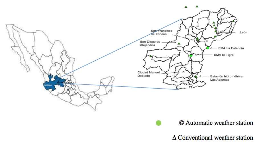
Table 1 shows the most important characteristics of the basin under study. The rains and their floods that have occurred since the 1970s have resulted in flooding in the municipalities of southwestern Guanajuato and caused damage in aspects such as health, property damage, interruption of economic activities and agricultural losses. The major floods so far of this millennium occurred in 2003 and 2007; therefore, in this work the rainfall-runoff behavior of the rainfall event that occurred from July 24 to July 31, 2007 was simulated, since detailed data of storms recorded by automatic weather stations (AWSs) are required to calibrate the model (Table 2). The floods of 2003, although they were more severe than those of 2007, were not modeled because this technology was not yet available in the basin.
Table 1 Characteristics of the Turbio River basin, Guanajuato, Mexico.
| Characteristic | Description |
|---|---|
| Area | 3,290 km2 to the “Las Adjuntas” hydrometric station |
| Average basin slope | 9.20 % |
| Main channel slope | 0.57 % |
| Main channel length | 118 km |
| Time of concentration | 19 hours |
| Dominant soil textural class | Fine 56 % and medium 33 %, of total area |
| Average annual rainfall in the entire basin | 659 mm (89 % of precipitation concentrated between June and October) |
| Rainy years-total rainfall (Reference station “El Palote”) | Year 2003 - 1,058 mm Year 2007 - 825 mm |
| Peak historical flows at the “Las Adjuntas” station (Comisión Nacional del Agua [CONAGUA], 2012) | 149 m3·s-1, September 21, 1971 130 m3·s-1, September 17, 2003 51.7 m3·s-1, July 28, 2007 |
Table 2 Rainfall depth in the Turbio River basin from July 24 to 27, 2007.
| Station | Rainfall depth (mm) | Rainfall five days before (mm) |
|---|---|---|
| 11020 | 143.9 | 9.0 |
| 11023 | 103.1 | 15.0 |
| 11025 | 89.6 | 24.5 |
| 11036 | 72.3 | 15.8 |
| 11040 | 149.6 | 15.0 |
| 11045 | 99.8 | 30.0 |
| 11055 | 141.7 | 17.1 |
| 11095 | 99.3 | 35.4 |
| 11159 | 104.1 | 6.2 |
| 14084 | 115.1 | 16.5 |
| 14123 | 151.6 | 11.7 |
| 14320 | 92.1 | 28.8 |
| 14369 | 119.8 | 4.0 |
| “Agroeduca” AWS1 | 70.4 | 20.2 |
| “La Estancia” AWS | 43.8 | 11.8 |
| “El Tigre” AWS | 37.2 | 7.4 |
| Average | 114 | 17.4 |
1AWS: automatic weather station.
The various rainfall-runoff model options developed in this work were carried out in the HEC-GeoHMS (USACE, 2013) and HEC-HMS (USACE, 2000, 2010a, 2010b) programs. The basin model and its physical parameters were obtained with the HEC-GeoHMS geotechnical extension designed for ArcGIS 10.1 (Environmental Systems Research Institute [ESRI], 2012), and were executed with the rainfall information represented through 13 hyetographs spatially distributed in the Turbio River basin with the Thiessen polygons method. These hyetographs fed the model at 1-h intervals. On average, the rainfall event of the evaluated period was 114 mm, the minimum value was 72 mm and the maximum 152 mm (Table 2).
For the event studied, three rainfall-runoff model alternatives were executed. In all three, the conversion of rainfall depth to direct runoff depth was carried out with the CN methodology. The methods that varied among the models were: a) the transformation of runoff depth to a direct runoff hydrograph (unit hydrograph or kinematic wave) and b) flood routing in channels (Muskingum or kinematic wave). In order to compare the predictive capacity of the models, three different combinations were made: 1) unit hydrograph-Muskingum (UH-Musk), 2) kinematic wave-Muskingum (KW-Musk) and 3) kinematic wave-kinematic wave (KW-KW). The three model alternatives executed the flood routing in the dams located in the Turbio River basin. These variants were developed in HEC-HMS and generated a hydrograph at the exit of the "Las Adjuntas" station.
Kinematic wave theory in a rainfall-runoff model
The KW model uses physical parameters to characterize a basin and takes the net rainfall or runoff depth as input to predict the flow. Miller (1984) presents the complete derivations of the Saint Venant equations (continuity [Equation 1] and motion [Equation 2]) applied to runoff modeling with KW, of which the final results are:
where Q = discharge, A = cross-sectional flow area, t = time, x = horizontal distance, y = depth, v = flow velocity, g = gravitational acceleration, S 0 = bed slope and S f = friction slope. Equation 2 is the one-dimensional form of the equation of motion that describes the non-permanent flow in open channels without lateral inflow.
To apply KW theory, it is assumed that the surface wave is long and flat, so that the friction slope is approximately equal to the bed slope. Then, the remaining terms of the equation of motion, also called secondary terms, are considered negligible; this implies that there is a balance between gravitational and frictional forces:
The KW model is based on the continuity equation and only approximates the dynamic equation with a uniform-flow equation. When defining the friction slope with the uniform-flow formula, the equation can be applied to a specific current or to a surface flow plane in the following way:
where α and m are defined coefficients for each cross section. Usually in the application of KW theory, Equations 5 and 1 are known as KW and are solved simultaneously.
According to Guo (1998) and Singh (1996), the numerical method to obtain the overland KW flow requires converting an irregular basin to a rectangular plane with equivalent slope. Among the necessary parameters of the basin, the width of the plane is a prerequisite for the numerical modeling of runoff (Guo, 1998).
MacArthur and DeVries (1993) stipulate that a critical parameter in the description of overland flow is the maximum length of the route taken by a drop of water to reach a current (Lw). The proper choice of Lw is vital as it determines the characteristics of the overland flow response. For its part, the Storm Water Management Model (SWMM; Rossman, 2010) manual suggests that the initial estimate of Lw is given by the basin area divided by the average maximum overland runoff length; subsequently, the model needs to be calibrated to confirm the selection of the KW plane width and other parameters.
The HEC-HMS includes all the models used in this work. In the KW model, there is the option to simulate a single plane, either of natural or urbanized areas, or two planes, when the sub-basin contains the two types of areas. The length of the HEC-HMS interface is the Lw of the KW plane.
Information used in the three models
To generate the basin model, the Mexican elevation continuum 3.0 (Instituto Nacional de Estadística y Geografía [INEGI], 2013), which has a resolution of 15 m, was taken as a base, and the geoprocessing tool included in the freely-available Geospatial Hydrologic Modeling Extension (USACE, 2013) for ArcGis was used. Through the transposition of the basin model, with the land-use and vegetation vector dataset, series IV scale 1:250,000 (INEGI, 2010), and the edaphologic vector dataset, scale 1:250,000 series II (INEGI, 2007), the CNs were obtained by sub-basin, which were corrected with the slope and rainfall of the previous five days (McCuen, 2016; Neitsch, Arnold, Kiniry, & Williams, 2009). Additionally, to perform the simulation with KW, it is necessary to know the cross-sectional area of the currents, which was obtained in the field. The parameter Lw was obtained by calculating the typical run distance of the runoff within each sub-basin. For this purpose, we determined the average of 10 measurements, from the limit of the sub-basin to the current, trying to include the diversity of distances by sub-basin. In the case of sub-basins that include both natural and urbanized areas, a value of Lw is calculated for each one, since two runoff planes are generated.
The Manning number for channel flow (n) and the effective resistance parameter for overland flow (N) were obtained from Chow, Maidment, and Mays (1988) and MacArthur and DeVries (1993), respectively. The information of the rainfall depth hyetographs was established from the information of the AWSs. The 24-h rainfall data reported in the conventional weather stations was used to have greater hyetograph coverage. The data were distributed over time according to the pattern presented in the AWSs, and spatially based on their area of influence, defined by the Thiessen polygons.
Model calibration
The quantitative measure of the goodness of fit between the simulation results and observed discharge is called the objective function and is equal to zero if these are identical. The objective function of minimum errors is reached when the values of the parameters that best reproduce the measured hydrograph are found (USACE, 2010b).
Among the objective functions offered by the HEC-HMS are those that minimize the root mean square error (RMSE). However, when it comes to minimizing the prediction error in peak flows, it is recommended to use the peak-weighted RMSE objective function, which is a modification of the standard RMSE function, which gives greater weight to flows above average and less weight to those below average (Cunderlik & Simonovic, 2004; USACE, 2010b). Therefore, in this work, when calibrating the following error function is minimized:
where PWRMSE is the objective function to minimize peak-weighted RMSE,
Q
t
sim
and Q
t
obs
are the flows simulated and observed at time t,
N is the number of observations in the period considered
and
Once the reported simulations were carried out, the necessary parameters were calibrated to obtain a better fit, taking as reference the hydrograph measured in "Las Adjuntas." To calibrate, both the CN and some flood routing parameters (Muskingum or KW) were used. After different tests, it was more useful to calibrate the models by fitting the CN for each sub-basin in a range of ± 10 %, a common practice among modelers (Arnold et al., 2012). The HMS model of the Turbio River presented in this work has 43 sub-basins.
Finally, at the moment that the HEC-HMS minimized the errors, between the simulated and observed values, only the curve numbers of 17 sub-basins were varied in UH-Muskingum and KW-Muskingum. In the UH-Musk model, the largest CN fit was -10 %, but on average they varied -6 %, and in the KW-Musk, the largest fit was -13 %. In the KW-KW model, the best CN fit achieved was -3 % in eight sub-basins, since when the fit was made in the same sub-basins as in the previous ones the results worsened.
An important guide to calibrate the models was the sensitivity analysis provided by the model. For example, when calibrating the UH-Muskingum model, it was observed that when a parameter does not provide improvement in the objective function it reports a value of 0.0. In Table 3, it is observed that when the CN of sub-basins W840 and W860 is varied, an improvement in the objective function is not reported, while in sub-basins W580 and W490 the CN improves the objective function.
Table 3 Sensitivity analysis of the runoff curve parameter in several sub-basins of the model in the unit hydrograph-Muskingum simulation.
| Sub-basin | Original CN1 | Calibrated CN | CN fit (%) | Sensitivity of the objective function |
|---|---|---|---|---|
| W560 | 80 | 75.3 | -5.9 | 0.47 |
| W580 | 76 | 69.7 | -8.2 | 1.48 |
| W490 | 78 | 70.5 | -9.6 | 0.81 |
| W510 | 76 | 68.4 | -10.0 | 0.17 |
| W710 | 71 | 66.8 | -5.9 | 0.33 |
| W730 | 73 | 70.1 | -4.0 | 0.42 |
| W680 | 62 | 59.5 | -4.0 | 0.18 |
| W620 | 68 | 65.3 | -4.0 | 0.08 |
| W750 | 63 | 60.5 | -4.0 | 0.25 |
| W760 | 61 | 58.6 | -4.0 | 0.18 |
| W630 | 66 | 60.9 | -7.8 | 0.40 |
| W600 | 56 | 53.8 | -4.0 | 0.05 |
| W610 | 57 | 54.7 | -4.0 | 0.13 |
| W640 | 68 | 61.2 | -10.0 | 0.16 |
| W650 | 56 | 51.4 | -8.2 | 0.96 |
| W670 | 61 | 58.6 | -4.0 | 0.25 |
| W690 | 58 | 54.6 | -5.9 | 0.25 |
| W840 | 54 | 51.8 | -4.1 | 0.00 |
| W860 | 47 | 47.0 | 0.0 | 0.00 |
1CN: runoff curve number.
According to Moriasi et al. (2007), the quality of a hydrologic model can be evaluated based on the value taken by the Nash-Sutcliffe efficiency index (NSE) (Table 4).
Table 4 Evaluation of hydrologic models according to Moriasi et al. (2007).
| NSE1 < 0.5 | Unsatisfactory model |
| 0.5 < NSE < 0.65 | Satisfactory model |
| 0.65 < NSE < 0.75 | Good model |
| 0.75 < NSE < 1.0 | Very good model |
1NSE: Nash-Sutcliffe efficiency index.
Additionally, the percent bias (PBIAS), which measures the average tendency of the simulated data to be greater or less than the observed values, was calculated (Moriasi et al., 2007):
A PBIAS of 0.0 indicates a very accurate model; if the value is positive it indicates that the model underestimates and if it is negative that the model overestimates. According to Moriasi et al. (2007), a PBIAS of less than 15 % is desirable when calibrating flows. However, Cunderlik and Simonovic (2004) mention that at the time of calibrating an hourly-type hydrograph, the lowest flows affect the PBIAS, and it is more desirable that there is no such bias in the largest flow values when it comes to a flood warning.
Results and discussion
Figure 2 shows the hydrographs resulting from the three simulated model alternatives; the one that presents the values obtained from the "La Adjuntas" station shows a peak flow of 51.7 m3·s-1 on July 28 at 4:00 p.m. This hydrograph is the benchmark for comparison with the three simulated models. In this sense, the KW-Muskingum method gives better results; however, the KW-KW model is the best at predicting the time at which the peak flow occurs, although it has the greatest error in volumes.
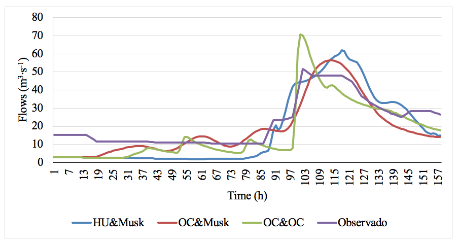
Figure 2 Hydrograph of simulated and observed flows from July 24 to 30, 2017 at the "Las Adjuntas" station of the Turbio River, Guanajuato, Mexico.
Table 5 shows the observed and simulated peak flows for each of the methodologies used. In this work, the UH-KW combination is not presented because the NSE reported values of -0.20, which is not acceptable.
Table 5 Peak flows of the simulations.
| Method | Peak flow (m3·s-1) | Hydrograph base time (h) | Peak time (h) |
|---|---|---|---|
| Observed hydrograph | 51.7 | 155 | 4:00 pm, July 28, 2007 |
| Unit hydrograph-Muskingum | 62.0 | 155 | 8:00 am, July 29, 2007 |
| Kinematic wave-Muskingum | 56.4 | 155 | 3:00 am, July 29, 2007 |
| Kinematic wave-kinematic wave | 70.8 | 155 | 4:00 pm, July 28, 2007 |
Table 6 shows the fits of the surface hydrologic model for the three methodological combinations, in addition to the statistics to choose the best model. According to the NSE, all three models are satisfactory (Moriasi et al., 2007). The best combination for the Turbio River rainfall-runoff model is the KW-Musk one, and the worst is the UH-Musk method. In the best methodological combination, the conversion of runoff depth to a hydrograph (flow) was made with the KW approach and the flood routing in channels with the Muskingum method, although it can be seen that the most used methodology in Mexico (UH-Muskingum) also shows a good fit, although of lower quality. In reality, the UH-Muskingum combination is preferred in Mexico because it is easier to have data available to feed the hydrologic model.
Table 6 Efficiency indices obtained in the three models.
| Method* | NSE1 | r2 | PBIAS (%) | RMSE (m3·s-1) | Residual error in volume (mm) |
|---|---|---|---|---|---|
| Unit hydrograph-Muskingum | 0.514 | 0.92 | 17.9 | 9.1 | -0.66 |
| Kinematic wave-Muskingum | 0.709 | 0.84 | 15.3 | 7.1 | -0.57 |
| Kinematic wave-kinematic wave | 0.582 | 0.83 | 23.0 | 8.5 | -0.87 |
1NSE: Nash-Sutcliffe efficiency index; r2: coefficient of determination; PBIAS: percent bias; RMSE: root mean square error.
*In all three methods, the hourly rainfall depth is converted into runoff depth with the runoff curve number.
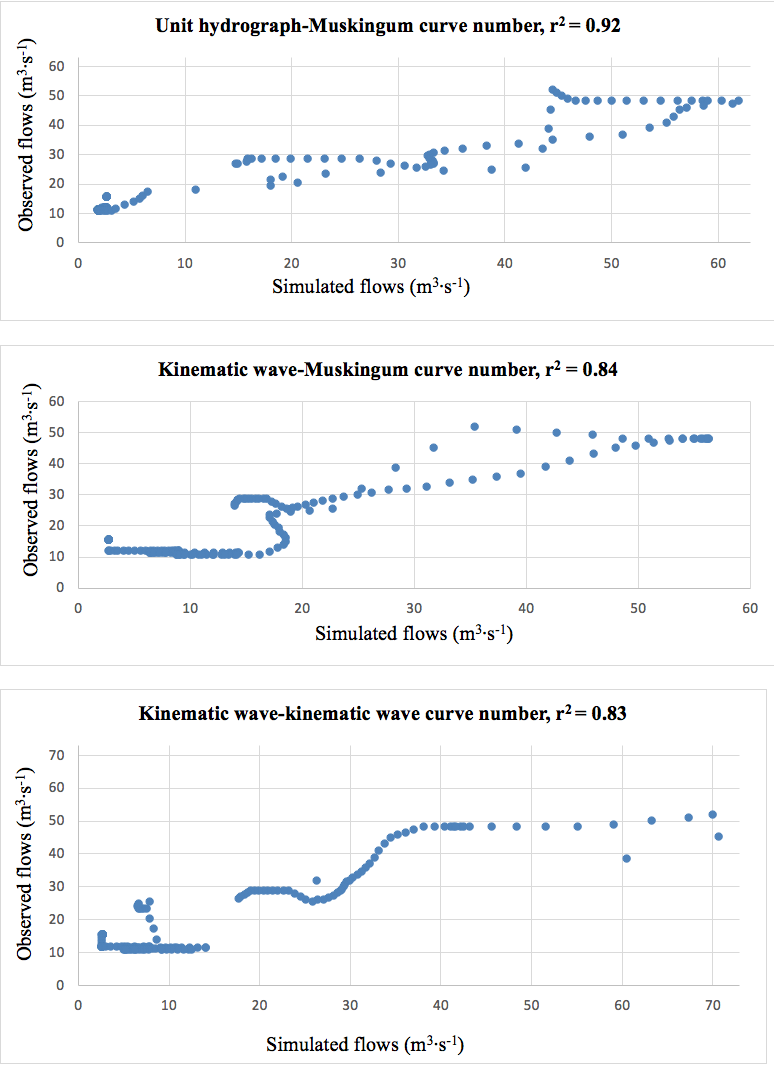
Figure 3 shows the dispersion behavior of the simulated flow predictions. In the KW-Muskingum and KW-KW methodologies, the simulated values present more error when it comes to predicting small flows, so that their r2 is lower than that of the UH-Muskingum method since the error occurs in small flows.
Conclusions
The best simulation of the rainfall-runoff process in the Turbio River basin is given by the kinematic wave-Muskingum combination; that is, the runoff depth becomes a hydrograph with the kinematic wave model and flood routing in channels is carried out with the Muskingum method. The Nash-Sutcliffe efficiency index obtained with this model was 0.709, which is considered good. The second-best simulation was with the kinematic wave-kinematic wave model, and the third with the traditional unit hydrograph-Muskingum.
According to the Nash-Sutcliffe coefficient, the three methods give satisfactory results, but the kinematic wave-Muskingum combination gives better results in terms of errors when estimating total flows, peak flow and runoff volume.

