


 texto en
  Inglés (pdf)
 Artículo en XML
 Referencias del artículo
 Enviar artículo por email
 Citado por SciELO
  Similares en
SciELO
Similares en
SciELO 
 Permalink
Introduction
The Humaya main channel (HMC), opened on October 8, 1952, belongs to Culiacán-Humaya Irrigation District 010 and is one of the most important in Mexico. It is located in the central region of the state of Sinaloa, passing through the municipalities of Culiacán, Navolato, Mocorito, Angostura and Salvador Alvarado. The district has a current irrigated area of 212,374 ha, of which 106,835 ha belong to ejidos and 105,539 ha to small properties (Comisión Nacional del Agua [CONAGUA], 2005). For administrative purposes, the district is organized into 12 irrigation modules, of which six are supplied by the HMC (Figure 1).

Figure 1 District 010 irrigation modules that supply the Humaya main channel (Pedroza-González & Hinojosa-Cuéllar, 2014).
The HMC is supplied by the Adolfo López Mateos dam, is 156 km long and has a large number of structures (26 reservoirs, a 1,310-m-long tunnel and 12 dikes; Pedroza-González & Hinojosa-Cuéllar, 2014). During its construction, in order to maintain depressions and take advantage of the runoff of some of the streams that cross the HMC, dikes were placed at different points along the channel (Table 1), whose initial capacity was determined with the volume that can be stored at different elevations depending on the channel’s operating levels.
Table 1 Dikes of the Humaya main channel, including cumulative distance and length.
| Dike number | Cumulative distance (channel) | Length (m) | |
|---|---|---|---|
| Entrance km | Exit km | ||
| 1 | 13+240 | 13+536 | 296.30 |
| 2 | 14+388 | 15+213 | 824.12 |
| Batamote | 35+678 | 36+696 | 1,018.06 |
| Arroyo Prieto | 37+120 | 37+630 | 510.00 |
| Agua Fría | 42+255 | 42+710 | 455.17 |
| Hilda | 43+539 | 43+851 | 312.33 |
| Mariquita | 52+311 | 56+851 | 4,539.51 |
| Palos Amarillos | 96+390 | 96+775 | 385.00 |
| Acatita | 99+130 | 100+380 | 1,250.00 |
| Cacachila | 138+632 | 139+169 | 537.31 |
| Aeropuerto | 155+950 | 156+911 | 961.00 |
Several studies, both geotechnical and hydraulic, have been carried out in the HMC, highlighted by the work conducted in 1997 with increasing the height of the banks in the first 5 km of the channel and in some intermediate-level sections, as well as cleaning work, water lily control in the lateral lagoons belonging to the dikes and expansion of reservoirs to increase their hydraulic area (Instituto Mexicano de Tecnología del Agua [IMTA], 1997). However, the bathymetry of the dikes has not been updated in the last fifty years and various factors have decreased their volumetric capacity, such as sediment and aquatic weeds (Camarena-Medrano & Aguilar-Zepeda, 2012).
Some authors indicate that the lack of maintenance in the HMC (such as sediment removal) causes 2.5 % losses in its conduction (Vargas & Pedroza, 2000). It is important to mention that poor sediment management can cause flooding, pollute the water supply and result in crop losses, among other problems. Therefore, it is necessary to carry out adequate conservation tasks to maintain the original storage capacity of each dike, avoiding or reducing the accumulation of sediment in the areas of preferential circulation.
A necessary task in quantifying sediment is bathymetry (Brock, Wright, Clayton, & Nayegandhi, 2004), which consists in determining the relief at the bottom of waterbodies (lakes, reservoirs and dikes) (Planella-González, Gómez-Pivel, & Alcoba-Ruiz, 2013). It is done by collecting the coordinates (x, y, z) of points distributed along the length and width of the waterbody, where x, y correspond to the location on the horizontal plane and z to the depth (being in turn the one that presents the greatest complexity; Farjas-Abadía, 2005). The latter has given rise to the development of sounding techniques.
Until the beginning of the last century, the most efficient sounding techniques involved physical contact using poles or ropes with lead, which posed major drawbacks. In the 1920s, work began on acoustic echo measuring equipment, which no longer required physical contact with the water bottom and streamlined the measurement process. Currently, acoustic Doppler current profilers (ADCP) are used to perform depth measurements, while incorporating a geolocation device to acquire the coordinates (x, y). These devices allow performing bathymetric surveys quickly and accurately, being an alternative to the traditional methods that determine the planimetry and altimetry separately (Farjas-Abadía, 2005). With the ADCP it is possible to obtain, among other estimates, the shape of the section, the speeds in the three dimensions and the flow of the channels with great precision (Hiebl & Musso, 2007; Leu & Chang, 2005).
Recently, conservation activities in the HMC made it necessary to determine the bathymetry of the dikes that make up the channel's conduction system. The HMC was designed to conduct a flow of 100 m³∙s-1; however, until 2013, the maximum that had been transported was 85 m³∙s-1. Since then, the freeboard has been reduced for the channel’s operation, disabling the flood works and allowing free flow in the floodgates. To increase the channel’s flow, by increasing the height of the dike walls, a review of the new operating conditions, including all the dikes installed, is required.
Therefore, the objective of this work was to determine the bathymetry of the HMC dikes using an acoustic Doppler current profiler to estimate the volumetric capacity, the flooded area and the maximum depth of each dike. The results were compared with the volumetric capacities published in 1997.
Materials and methods
Acquisition of coordinates and depth measurements
The coordinates (x, y, z) of the bathymetric study were determined with an acoustic Doppler current profiler (ADCP; model M9, SonTek brand) (Figure 2) with an accuracy of 1 % of the mean value and a resolution of 0.001 m, using a 0.5 MHz ultrasonic transducer. This instrument calculates the water velocity components in different layers in the three directions. As its name implies, this equipment uses the Doppler effect, as it transmits sounds at a fixed frequency and captures the echoes returned by water reflectors (Lee, Mukai, Lee, & Lida, 2008). The reflectors are small microscopic particles of sediment or plankton present naturally in water (Hiebl & Musso, 2007). When the sound sent by the ADCP reaches the reflectors there is a frequency displacement proportional to the relative speed between the ADCP and the reflectors. Part of the sound is reflected once again to the ADCP. This second displacement is used to calculate the speeds (Figure 3).
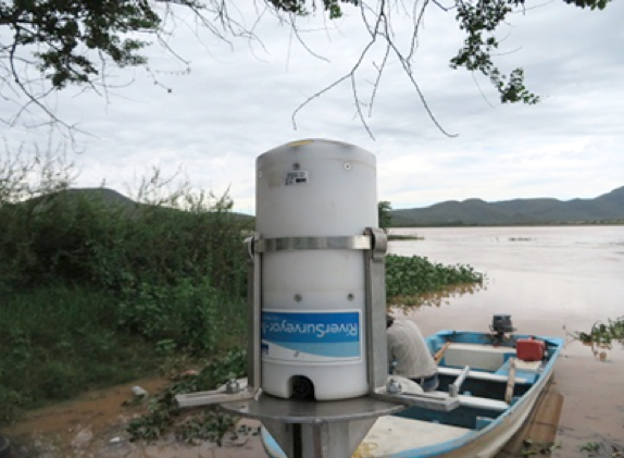

Figure 3 Operating principle of an acoustic Doppler current profiler (ADCP). Adapted from Muste, Kim, and Fulford (2008).
As a backup measure, the coordinates (x, y) were also captured with real-time kinematic (RTK) satellite navigation equipment. The equipment used was of the Topcon brand, with horizontal resolution of 10 mm + 1.0 ppm and has support for various systems, such as GPS, GLONASS, QZSS (Quasi-Zenith Satellite System), SBAS (Satellite Based Augmentation System) and Galileo. The RTK improves the precision of other positioning systems, such as the use of the Global Positioning System (GPS) or the Differential GPS (DGPS), allowing high-precision readings in real time, even if the receiver is in motion (Langley, 1998). An RTK consists of two stations, one static (reference) and the other mobile. The latter contains the movement receiver with which the coordinates will be determined in real time (with the option to do so in the local reference system). The reference station provides instantaneous corrections for the mobile station (Paar, Novakovic, & Kolovrat, 2014).
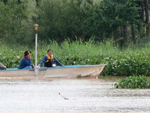
To perform the reading of the coordinates in each dike, the ADCP and the RTK were mounted on a motor boat (Figure 4). In general, a tour was made along the edge of the dike, sweeping every 20 m in both directions. This allowed the collection of points that associate the depth levels with the position within the dikes. As an example, in Figure 5 the route and the position of the sampled points in Dike 1 were schematized. The equipment was programmed to perform the automated capture of the coordinates: ADCP every 4 s and RTK every 10 s.

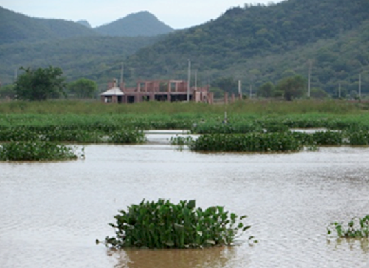
Some dikes exhibited problems of floating and emergent weeds in a partial (Figure 6) or even total manner, which limited the scope of the sweeps. Therefore, in the Arroyo Prieto, Hilda, Mariquita, Palos Amarillos, Acatita, Cacachila and Aeropuerto dikes it was difficult to cover the entire surface. On average, 20 % of the area (mainly on the edge of the dikes) was unfathomable.
Construction of the bathymetric models
The depth and position data obtained were reviewed and analyzed with Google Earth and Esri ArcGis Desktop. The Google Earth application provided a first visual approximation to the location of the points, which allowed detecting that in three dikes there was an offset of the coordinates (x, y), possibly due to a calibration error of the compass. The points with deviations were corrected based on the RTK backup information, with the ArcGis Desktop program using the timestamp readings to make the correlation. Once the information was integrated, a table with the coordinates (x, y, z) of each dike was obtained.
To construct the models, the coordinates were introduced into the Surfer program. This application allows building contour maps and digital elevation models from the interpolation of the points x, y, z by means of a process called "gridding." Surfer offers various algorithms for this task. In this work we used the Kriging algorithm (Goovaerts, 1997), which is considered the best interpolation method for spatial data (Jassim & Altaany, 2013). Kriging predicts the value of a spatial attribute in a particular location of already known positions, taking into account spatial dependence and autocorrelation (Bhattacharjee, Mitra, & Ghosh, 2014). Unlike other methods, Kriging attempts to express trends suggested by the data, so that, for example, the high points are connected along a ridge rather than isolated by circular contours (Yang, Kao, Lee, & Hung, 2004). The basic form of the Kriging estimator is (Jassim & Altaany, 2013):
where P i are the observed points, λ i is the weighting factor for each point i and P* is the point that we want to estimate. Therefore, the purpose of the estimator is to determine the weights λ i that minimize the variance, considering that:
E{P*- P} = 0
and
Typically, the weights λ i are constructed by means of a variogram (whether linear, spherical, or exponential), which describes the spatial behavior of the variable z (Kerry & Hawick, 1997). For this work, the model used was linear with slope equal to one and without anisotropy. This option and parameters are selected by definition in the Surfer program for the execution of the Kriging algorithm. The output for the Kriging method is a file containing data x,y,z in grid format (file.grd), which correspond to the interpolated coordinates of the entire gridding region. The z values greater than 0, obtained by the trends detected in the interpolation, were eliminated.
The delimitation of the regions of interest was done with vector maps constructed in the ArcGis Desktop program, using as reference Google Earth images and points acquired with the RTK at the ends of the dikes. These points also allowed establishing the upper elevation in masl. For their presentation, contours with a separation of 20 cm were obtained. The volumes were also calculated with the Surfer program, which uses the numerical integration to perform the calculation, specifically Simpson's 3/8 rule. Finally, a digital elevation model (DEM) of each dike was obtained.
Results and discussion
The contours and the DEM (Figure 7) allowed obtaining the area and volume data for each elevation. This information allowed generating the elevation-area-capacity graphs of each dike. Figure 8 shows the graph of dike 1, showing the increase in volume (red curve, lower horizontal axis) and area (blue curve, upper horizontal axis) as a function of depth (vertical axis). For convenience, this last datum is expressed in masl, reaching the bottom at 64.8 masl and the water mirror at 72 masl, giving a depth of 7.2 m. The graph allows quickly identifying the volume and coverage area as a function of the height reached by the water in the dikes.

Figure 7 Contours (a) and digital elevation model (b) resulting from the bathymetry of dike 1. Author-made with data obtained from the measurement of dike 1.
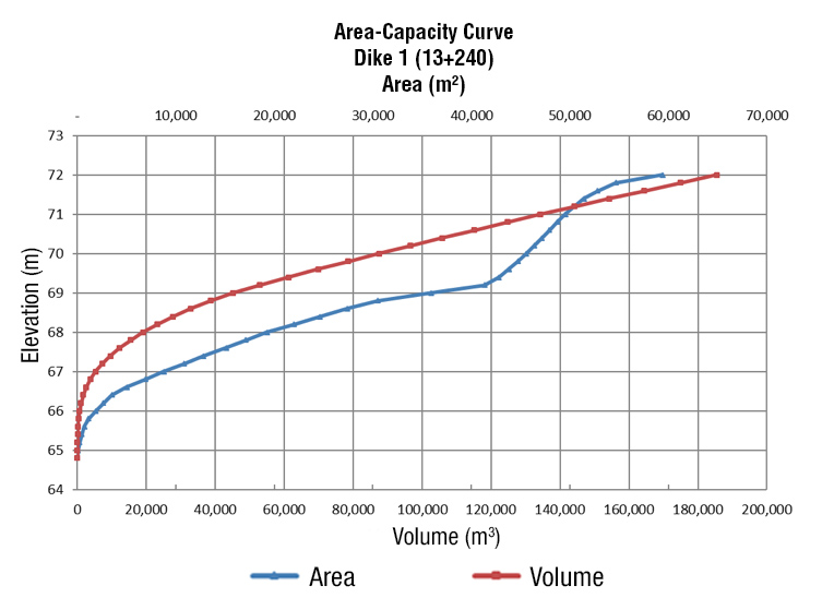
Table 2 shows the main product of the work carried out, which are the volumetric capacity (m3), flooded area (ha) and depth (m) data of all the HMC dikes, even those that could not be sounded in their entirety due to aquatic weed problems (4 of the 11 dikes).
Table 2 Volumetric capacity, flooded area and depth at sediment level of the HMC dikes.
| Dike | Volumetric capacity (m3) | Flooded area (ha) | Depth (m) |
|---|---|---|---|
| 1 | 185,460 | 5.41 | 7.20 |
| 2 | 706,905 | 227.84 | 7.50 |
| Batamote | 4,414,376 | 130.00 | 9.50 |
| Arroyo prieto* | 1,020,000 | 33.00 | 7.80 |
| Agua fría | 268,951 | 15.60 | 5.60 |
| Hilda | 135,522 | 13.55 | 5.75 |
| Mariquita | 15,255,513 | 445.47 | 11.5 |
| Palos amarillos* | 495,667 | 22.83 | 4.25 |
| Acatita* | 750,000 | 42.00 | 4.20 |
| Cacachila | 1,223,892 | 69.00 | 4.60 |
| Aeropuerto* | 977,406 | 76.72 | 3.35 |
*dikes not fully studied due to aquatic weed problems.
Table 3 shows the volumes of each dike compared to those originally calculated in 1966 (IMTA, 1997). To make a proper comparison, the same elevation was used in the curves of both bathymetries, excluding dikes that were not fully covered due to the problem of aquatic weeds. Negative values denote a loss of volumetric capacity. As can be seen, dikes 1 and 2 increased their capacity, due to the maintenance and expansion work that was recently carried out. On the other hand, Batamote, Agua fría, Hilda, Mariquita and Cacachila were those that showed the greatest loss of capacity, most likely due to the sediment. This is important since it is estimated that, on average, the economic losses worldwide due to the reduction of storage capacity for irrigation due to sediment are in the range of 3 to 5 billion dollars per year (International Commission on Large Dams [ICOLD], 2010).
Table 3 Comparison of the volumetric capacity between the 2013 and 1966 bathymetric surveys.
| Dike | Elevation (z) | Bathymetry 2013 (m3) | Bathymetry 1966 (m3) | % decrease (-) or increase in volumetric capacity |
|---|---|---|---|---|
| 1 | 72.00 | 185,460.04 | 153,931.03 | 20.48 |
| 2 | 72.00 | 706,905.66 | 637,221.14 | 10.94 |
| Batamote | 68.00 | 4,414,376.82 | 5,575,147.84 | - 20.82 |
| Agua Fría | 66.00 | 241,774.27 | 292,500.00 | - 17.34 |
| Hilda | 66.00 | 349,356.83 | 400,000.00 | - 12.66 |
| Mariquita | 63.00 | 11,385,259.06 | 15,700,000.00 | - 27.48 |
| Cacachila | 49.00 | 1,223,891.17 | 1,302,325.58 | - 6.02 |
Conclusions
The dikes of the Humaya main channel are operated as a function of the channel’s level and serve as temporary water storage areas in the case of normal flow. In this way, the dikes function as buffers against probable extraordinary contributions, flood flow and floodgate movements, as well as deposits of irregular volumes. Therefore, the dikes act as a protection and buffering system for the CPH, which makes their conservation and timely maintenance extremely important.
An acoustic Doppler current profiler is an extremely useful tool for obtaining the depths of dikes. From its use it was possible to determine the volumetric capacity of the HMC dikes. However, its use was limited by the presence of aquatic weeds and excessive sediment accumulation. For this reason, only seven of the eleven dikes could be sounded correctly.
Of the seven dikes that were almost completely studied, the comparison showed that two increased their capacity due to the correction made in the channel’s main canal. In the remaining five there was no accumulation of sediment, which caused, on average, a 16.87 % decrease in their capacity. This shows the need to carry out an effective sediment control program in the most affected dikes.
Weeds and sediment obstruct the free flow of water through the dikes, causing load losses and significantly influencing the conduction and response capacity of the channel. Poor sediment management not only increases maintenance costs, but also causes significant losses to irrigation users.

