


 texto en
  Inglés (pdf)
 Artículo en XML
 Referencias del artículo
 Enviar artículo por email
 Citado por SciELO
  Similares en
SciELO
Similares en
SciELO 
 Permalink
Introduction
Forest ecosystems give goods and environmental services for human well-being like sources of food, medicines and biofuel, raw materials for construction, clean air and water, protection of soil and water, and vital wood supplies; they also help to mitigate climate change (Food and Agriculture Organization of the United Nations [FAO], 2020; Tidwell, 2016). Thus, these resources must be preserved; for this, one has to properly manage forest stocks to meet the broad-sense goal for satisfying social, economic, cultural and spiritual needs (Larrubia et al., 2017).
Over a number of meetings, researchers have established a set of criteria and indicators for determining the progress towards sustainable forest management at regional and national scales (Baycheva-Merger & Wolfslehner, 2016; Jalilova et al., 2012; Larrubia et al., 2017). These criteria and indicators cover seven thematic elements of sustainable forest management: extent of forest resources; biological diversity; forest health and vitality; three types of functions (protective, productive, and socio-economic), and legal policy and institutional frameworks (Jalilova et al., 2012; Larrubia et al., 2017). However, to complement the criteria and indicators information at the local scale, there is a need for objective, practical, and relatively cheap measures, as the one of sustained timber yield, which managers can adopt. Although it is true that an index or measure that estimates the recovery of stocks is affordable, one must always be vigilant of other changes in the forest since, as a multidimensional system, the measure cannot always fully capture them (Picard et al., 2012).
The sustained yield has been an accepted principle and a paradigm in forestry for a long time (Hahn & Knoke, 2010). Sustained yield is the ability of the forest to maintain its growth or production, in terms of volume and biomass, approximately at the same level or higher than its historical average (Dauber et al., 2005; Irland, 2010). The concept has evolved, but the original meaning is still pertinent and indirectly represents many relevant ecological processes that occur in the forest (Irland, 2010). Monitoring and assessing timber yield is important because they allow verifying that soil productivity, the amount of water, and other abiotic elements and living beings remain in good condition (Irland, 2010). Consequently, if there are indications that timber yield has not been sustained, this should lead to the implementation of appropriate management operations to mitigate forest degradation.
The recovery rates of volume stocks of trees have been used, after the felling period, to evaluate whether the timber yield has been sustained (Castro et al., 2021; Piponiot et al., 2018; Vidal et al., 2016). These evaluations require the availability of timber volume data during the harvesting period, from the beginning to the end, which generally come from permanent plots or forest inventories. However, it is necessary to have options to estimate whether the timber yield has been sustained when such data of inventory or permanent plots are not available. On the other hand, environmental conditions in forest ecosystems change rapidly and often vary before it is possible to verify the suitability of silvicultural practices (Anderson-Teixeira et al., 2013). One possible solution is to look at the system output to confirm the expected results and to verify if the environment remains in good condition, which is the ex-post approach of the procedure presented here.
The objective of this study is to propose a procedure to measure a posteriori whether the timber yield of a forest has been sustained over a wide time scale by tracking the heights and diameters reached by same-aged trees established in different years. Timber yield will be sustained if there is a sustainable forest, in the medium and long term.
Materials and methods
Study area
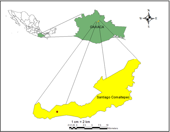
Data was chosen from a forest area with an extension of 18 070 ha in Santiago Comaltepec, Ixtlán de Juárez, Oaxaca, Mexico, to illustrate the procedure for tracking timber yield. It is a temperate forest with dominant presence of Pinus patula Schiede ex Schltdl. & Cham., mixed with Pinus oaxacana Mirov., Pinus pseudostrobus Lindl., Pinus ayacahuite Ehrenb. ex Schltdl., Quercus spp. and Arbutus spp. The forest is located in the Sierra Norte, between 96° 30’ 54.90“ and 96° 30’ 50.85” W and 17° 34’ 13.26” and 17° 34’ 6.32’’ N, at an altitude of 2 005 m (Figure 1).
From 1956 to 1982, the study area was under a concession to a papermaking company (Fábricas de Papel Tuxtepec), a time when all the wood of any species of Pinus was transformed into cellulose. Between 1956 and 1992, the wood was extracted under the Mexican Method of Forest Regulation (MMFR). The MMFR is based on the selective cutting of senile, plagued, sick, poorly shaped or standing dead trees, with a maximum pre-established cutting intensity of 35 % and a 25-year-cutting cycle; the aim is to convert over-mature forests to better productivity forests (Torres-Rojo et al., 2016). Subsequent to 1992, the Method for Silvicultural Development was adopted, using clearcutting in strips and seed trees as regeneration methods, enriched with planted seedlings (Roldán-Félix, 2014).
Sampling and tree grouping
A sample of 98 adult trees of P. patula was taken as representative for evaluating the growth of diameter and height of the trees, which are the main variables of volume estimation. Given the variation in the dimensions of the trees, they were grouped into four categories (Table 1): very big, big, medium and small. Tree grouping allows a valid comparison between them and serves as a control for covariates that were not observed over time. The ages of trees were only known after the stem analysis.
Table 1 Criteria for grouping trees of Pinus patula by height and diameter.
| Height category (m) | Diameter category (cm) | |
|---|---|---|
| Group 1 | Highest tenth part (35-36 m). | Highest fourth part (70-80 cm). |
| Group 2 | (i) Trees located in the tenth decile of the height category, which do not belong to the fourth quartile of diameters; (ii) trees in the fourth quartile of diameters which do not belong to the tenth decile of the height category; (iii) trees located in the ninth decile of the height category and in the third quartile of the diameter category. | |
| Group 3 | Trees that do not meet the criteria of groups 1, 2 or 4. | |
| Group 4 | Lowest tenth part (9-13 m). | Lowest fourth part (15-25 cm). |
Extremes: trees in the highest tenth of heights and the highest fourth of diameters form Group 1 of the biggest trees. In the contrast, trees in the lowest tenth of heights and the lowest fourth of diameters form Group 4 of smallest trees.
Some information about the establishment year of trees in each size group is required. The years were as follows: the biggest trees in Group 1 were established from 1903 to 1940 and trees in Group 2, from 1897 to 1941; in these groups, all the trees were born before the selective extraction of long-lived individuals which began in 1956. Trees in Group 3 emerged between 1902 and 1981, and only 12 out of 72 emerged after 1956. Finally, trees of Group 4 were born from 1937 to 1980, and 5 out of 8 emerged after 1956. Of the 98 trees sampled, five belong to Group 1 (very big), 13 to Group 2 (big), 72 to Group 3 (medium size), and 8 to Group 4 (small).
Measurement of diameters and estimation of heights
From the stem analysis data, the height (h δ ), of a tree at age δ = 10, 20,…, 70 was estimated by linear interpolation. For that, two ages were selected, one upper (u) and one lower (l), with both as close as possible to δ, through the following formula:
In this formula, h u : upper section height; h l : lower section height; A u : upper section age; A l : lower section age. To get the year when the tree reaches age δ, the establishment year (EY) is required, calculated by EY = CY ‒ A, where CY is the cutting year and A is the cutting age. For every tree, the value of h δ and the year when the tree reached it (y δ ) were recorded.
Diameters were measured directly from rings in each decade for the stump section (at a height of 0.35 m) and section 1 (at a height of 3.02 m), respectively. For the stump section, diameters were also measured when the trees were five years old.
Data analysis
The key idea of the procedure is to track stability in timber production, based on stem analysis data in which sampled trees established in different years were scaled at the same age to be compared. The procedure is easy, intuitive and viable to carry out in both natural forests and plantations, once the stem analyses are available. Furthermore, the proposal immediately signals the effects caused by disturbances in the forest and could therefore reveal whether silvicultural practices, such as thinning, controlled burning or logging, were properly managed. Growth ring data from P. patula trees sampled in a pine-oak forest, that has been managed by the Mexican Method of Forest Regulation and the Method for Silvicultural Development (Roldán-Félix, 2014; Torres-Rojo et al., 2016), were used to measure whether the timber yield has been sustained.
To assess a posteriori the timber yield sustainability, the diameter and height growth of same-aged trees (established in different years) grouped by size was monitored, using simple regressions. After that, a multiple regression over all the trees was carried out. All the regression analyses were carried out using the R statistical package (R Core Team, 2021).
Models for heights and diameters of same-aged trees grouped by size
Simple linear regressions of heights of trees that belong to the same category when they were of equal age (in decades) against the year when they reached that age were carried out.
The four groups of heights and the first three ones for diameters were analyzed because is expected that the smallest trees come from suppressed conditions, where the diameter growth is more affected (Olivar et al., 2013). For groups 1, 2, and 3, data were available at age δ = 10, 20,…, 70, and for Group 4, only four ages (δ = 10, 20, 30, 40) were available. The regression model for height was:
In this model, j = 1, 2, …, n δ , n δ is the number of trees at age δ and δ = 10, 20,…, 70; h δj = height of j-th tree at age δ; a δ = intercept for age δ; b δ = slope for age δ; y δj = year in which the j-th tree reaches the age δ, and e δj = error term. The parameter b δ represents the marginal growth of height with respect to the establishment year.
The hypothesis test carried out in each decade-group combination for the dependent variable height was:H 0 : b δ < 0 against the alternativeH a : b δ ≥ 0. If b δ ≥ 0, then, at age δ, the heights of more recently established trees are equal to or greater than those of the earlier established ones and would indicate that timber yield has been sustained; otherwise, if H 0 is not rejected, then there is evidence that timber yield has not been maintained. See Table 2 for the number of observations for each hypothesis test.
Table 2 Number of observations included in the models of the three studied variables of Pinus patula trees.
| Group | Age | Total by group | |||||||
|---|---|---|---|---|---|---|---|---|---|
| 5 | 10 | 20 | 30 | 40 | 50 | 60 | 70 | ||
| Heights | |||||||||
| 1 | - | 5 | 5 | 5 | 5 | 5 | 5 | 4 | 34 |
| 2 | - | 13 | 13 | 13 | 13 | 13 | 13 | 12 | 90 |
| 3 | - | 72 | 72 | 70 | 67 | 60 | 55 | 40 | 436 |
| 4 | - | 8 | 8 | 7 | 4 | - | - | - | 27 |
| Total by age | 98 | 98 | 95 | 89 | 78 | 73 | 56 | 587 | |
| Diameters at the stump section | |||||||||
| 1 | 5 | 5 | 5 | 5 | 5 | 5 | 5 | 4 | 39 |
| 2 | 13 | 13 | 13 | 13 | 13 | 13 | 13 | 12 | 103 |
| 3 | 72 | 72 | 72 | 70 | 67 | 60 | 55 | 41 | 509 |
| Total by age | 90 | 90 | 90 | 88 | 85 | 78 | 73 | 57 | 651 |
| Diameters at section 1 | |||||||||
| 1 | - | 5 | 5 | 5 | 5 | 5 | 5 | 4 | 34 |
| 2 | - | 10 | 13 | 13 | 13 | 13 | 13 | 12 | 87 |
| 3 | - | 51 | 72 | 70 | 67 | 60 | 55 | 41 | 416 |
| Total by age | 66 | 90 | 88 | 85 | 78 | 73 | 57 | 537 | |
Examples to manage the table: For a simple regression on heights for group 2 and age 40, 13 observations were used; for multiple regression of diameter at the stump section, 651 observations were used.
Models for the diameters (stump section and section 1), as well as the interpretation of the coefficients, were analogous. For example, the diameter model at the stump section can be written as d δj (stump) = a δ + b δj y δj + e δj , where d δj (stump) represents the diameter at the stump section of the j-th tree at age δ, with δ = 10, 20,…, 70; the other elements of the model have a similar meaning as in the height model, but related with diameter at the stump section. The hypothesis test is also carried out on the parameter b δ , which in the model of diameter represents the marginal growth of diameter with respect to the establishment year.
Models for heights and diameters considering all trees
An additional analysis using all the trees in a model that implicitly grouped them by age δ was performed. This analysis also makes the hypothesis testing on c h stronger, due to the increase in the error degrees of freedom. The multiple regression model for height was:
with j = 1, 2, …, n
δ
and δ = 10, 20,…, 70; where y
δj
is the year when the j-th tree reaches the age δ, a
h
is a general intercept, b
h
is a parameter that relates height to age, and c
h
is a parameter of the marginal growth by year. Note that from a
h
and b
h
, a particular ordinate is obtained for each age δ,
The regression models for the diameters at the stump section and section 1, as well as the interpretation of the coefficients, are analogous. That is, the multiple regression model for diameter at the stump section of the j-th tree, with j = 1, 2, …, n
δ
, at age δ = 10, 20,…, 70, d
δj
(stump), was
A schematic representation of the steps to estimate whether the timber yield has been sustained is presented in Figure 2.

Figure 2 Schematic representation of timber yield monitoring. After having the heights and diameters, there are two alternatives to measure if timber yield is sustained: by tracking the heights and diameters reached by same-aged trees (established in different years) grouped by size or by tracking such dimensions considering all trees as a whole.
Forest manager interviews
Since management approach is relevant to preserve forest land, some forest managers were contacted to request their opinion on the forest development of the study area in the last 30 years, to compare them with the results obtained in this investigation. The questions were focused on the management of the forest, wood quality, composition of species and their general perception over changes in the forest.
Results
Patterns of heights and diameters of same-aged trees grouped by size
Height
In the height patterns of trees for group 2, clustered by decades (Figure 3), it is evident that all the slopes are positive and the slopes of the models for older trees are greater than those for the younger ones. This finding implies that more recently established trees not only grew faster, but their marginal growth were greater at 60 or 70 years old than at 10 or 20 years old.

Figure 3 Height growth trends grouped by decades for Pinus patula trees of Group 2. No tree age has a negative slope; thus, the average height is maintained, at least, as in the beginning of logging, and consequently, a forest deterioration did not happen. The fitted regression equations
Slopes for height models appears in Figure 4 for all groups and each decade within them. Non-negative trends are observed for all trees (Figures 4A, 4D, 4G, 4J). The corresponding P-values of the tests are in Table 3. Comparing the estimation of the slope value for each age in the four groups of trees, only one is negative but not significant; the rest of them are positive, half of these are highly significant, so the height dimension remains at the same level or bigger.
Table 3 Slopes and P-values for height models, by groups and decades of Pinus patula trees.
| Group 1 | Group 2 | Group 3 | Group 4 | |||||
|---|---|---|---|---|---|---|---|---|
| Age | Slope | P-value | Slope | P-value | Slope | P-value | Slope | P-value |
| 10 | 0.0732 | 0.1796 | 0.0392 | 0.3446 | 0.0005 | 0.9831 | 0.0118 | 0.7259 |
| 20 | -0.0052 | 0.9232 | 0.1399 | 0.0011 | 0.0308 | 0.1886 | 0.0628 | 0.0735 |
| 30 | 0.1186 | 0.0341 | 0.2037 | <0.0001 | 0.0485 | 0.0630 | 0.0210 | 0.5806 |
| 40 | 0.2002 | 0.0008 | 0.2043 | <0.0001 | 0.0541 | 0.0691 | 0.0407 | 0.5483 |
| 50 | 0.2199 | 0.0003 | 0.1940 | <0.0001 | 0.0365 | 0.4001 | ̶ | ̶ |
| 60 | 0.1429 | 0.0121 | 0.1792 | <0.0001 | 0.0952 | 0.0687 | ̶ | ̶ |
| 70 | 0.1549 | 0.0130 | 0.1642 | 0.0004 | 0.1332 | 0.0367 | ̶ | ̶ |

Figure 4 Slopes for heights and diameters for size groups of Pinus patula trees. Slopes look steeper in bigger trees. Slopes in diameter at the stump section seem similar to the ones at section 1 and slopes in heights and diameters of Groups 1 and 3 have some resemblance. Slopes for all variables indicate that more recently established trees had bigger dimensions. Significance codes: black circles indicate a significant test at 0.05 and 0.01; gray circles indicate that it was at 0.1, and open circles indicate no significance. The gray horizontal line signals zero.
The height patterns in Groups 1 and 2, to which the tallest trees belong, are very similar (Figures 4A and 4D). In Group 1 (Figure 4A), the biggest slope happened in the fifth decade, while in Group 2 (Figure 4D), it occurred in the fourth. The species reaches its maximum size around these ages. As an example of the tests of hypotheses on height for a specific age and group of trees, see Appendix 1. In Group 3, the positive slopes (Figure 4G) show a weak significant difference to zero between the decades 3 and 6, except the 5th.
Diameter
For the three groups of trees, section 1 has similar diameter slopes to the ones on the stump section (Figures 4B and 4C, 4E and 4F, 4H and 4I). As with the height’s development, the most recently established trees in Groups 1 and 2 had larger diameter increments; however, for Group 3, this trend is only observed in ages 60 and 70. This claim is supported by the statistical significance for the slopes in each section, group, and age, shown in Table 4; therefore, the dimensions of diameters both at stump section and section 1 remain at the same level or bigger. Regarding the value of the slope for each age in the three groups of trees analyzed, four of them are negative but not significant, except one at 10 years; this significance disappears in later ages. There are 18 positive slopes, of which 15 are highly significant. Regarding the value of the slope for each age in the three groups of trees analyzed, five of them are negative but not significant. There are 16 positive slopes, of which 12 are highly significant. Negative slopes are not significant at the 0.05 level, except for the stump section during the first decade.
Table 4 Slopes and P-values for diameter models, by section, group and age of Pinus patula trees.
| Group 1 | Group 2 | Group 3 | ||||||
|---|---|---|---|---|---|---|---|---|
| Age | Slope | P-value | Slope | P-value | Slope | P-value | ||
| Stump section (at 0.35 m) | ||||||||
| 5.0000 | 0.0463 | 0.7152 | 0.0234 | 0.7723 | -0.0246 | 0.5918 | ||
| 10.0000 | 0.2482 | 0.0574 | 0.1811 | 0.0275 | -0.0911 | 0.0480 | ||
| 20.0000 | 0.4151 | 0.0024 | 0.2649 | 0.0013 | -0.0891 | 0.0529 | ||
| 30.0000 | 0.4875 | 0.0005 | 0.2700 | 0.0012 | -0.0477 | 0.3507 | ||
| 40.0000 | 0.5641 | <0.0001 | 0.2687 | 0.0013 | 0.0010 | 0.9863 | ||
| 50.0000 | 0.5406 | 0.0002 | 0.2838 | 0.0007 | 0.0534 | 0.5306 | ||
| 60.0000 | 0.5098 | 0.0003 | 0.3328 | <0.0001 | 0.2790 | 0.0067 | ||
| 70.0000 | 0.5298 | 0.0006 | 0.4807 | <0.0001 | 0.3502 | 0.0052 | ||
| Section 1 (at 3.02 m) | ||||||||
| 10.0000 | 0.1932 | 0.1629 | 0.1076 | 0.2227 | -0.0629 | 0.2497 | ||
| 20.0000 | 0.3453 | 0.0162 | 0.2142 | 0.0139 | -0.0635 | 0.1657 | ||
| 30.0000 | 0.4715 | 0.0016 | 0.2321 | 0.0079 | -0.0429 | 0.3991 | ||
| 40.0000 | 0.5579 | 0.0003 | 0.2472 | 0.0048 | -0.0080 | 0.8907 | ||
| 50.0000 | 0.4360 | 0.0032 | 0.2379 | 0.0077 | -0.0052 | 0.9513 | ||
| 60.0000 | 0.4015 | 0.0060 | 0.2264 | 0.0095 | 0.1525 | 0.1355 | ||
| 70.0000 | 0.3449 | 0.0272 | 0.3707 | 0.0001 | 0.2130 | 0.0870 | ||
In Figure 5A, diameters clusters are presented for the stump section at all ages, for trees in Group 2. The slopes for trees in Group 1 are similar to Group 2 (Figures 4B and 4E). Figure 5B shows the fitted lines for diameter at the stump section for Group 3, which is the biggest conglomerate of trees. There is a smooth change in the slopes over time, from negative to positive, between decades 4 and 5; however, the magnitude of the positive slopes is greater than the negative ones (Figure 4H). Comparing the first three groups, slopes for heights and diameters were, in general, bigger in Group 1, followed by Groups 2 and 3 (Figure 4).

Figure 5. Estimated regression lines for diameter at the stump section for Pinus patula trees in Group 2 and Group 3. Patterns in trees of Group 1 are similar to the pattern in trees of Group 2. For Group 3, diameter patterns at section 1 are similar to the patterns of the diameter at the stump section. The majority of slopes in Groups 2 and 3 are statistically different from zero (most with a positive sign). The gray dashed vertical line indicates year 1956, when the extraction of trees started. y/o: years old.
Models for heights and diameters considering all trees
In the multiple regression model that includes all the trees, the estimated lines for heights, diameter at the stump section, and diameter at section 1 are, respectively:
From the general model of each variable, it can be generated a particular equation for each age; the corresponding equations for height and diameter at the stump section are in Figure 6. The diameter growth in the stump (Figure 6B) was similar to the diameter in Section 1.
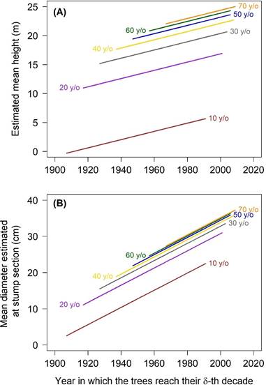
Figure 6 Estimated regression lines from the regression model including all the Pinus patula trees. (A) Regression lines for heights. (B) Regression lines for diameters at the stump section. In both cases, from the general fitting on all the trees, equations were generated for ages of 10, 20,..., 70 years old (y/o); the estimated general mean (intercept) increases as age increases and the slopes are positive.
The relevant hypothesis testing is on the year parameter related with the variable y δj , whose results are presented in Table 5. Both the individual tests (Table 5) and the respective joint tests, for the three response variables of interest, are highly significant. Appendix 2 shows an example of the height hypothesis test for the model that includes all trees, regardless of size grouping. Tests for diameters were done in a similar way.
The results of comparing diameters and height of same-aged trees coincide with those that managers know about the forest development during the time involved. In addition, managers agree that species composition and densities have been approximately at same level.
Table 5 Individual hypothesis tests on the year parameter, for heights and diameters of Pinus patula.
| Response variable | Year estimate | Standard error | t value | Pr(>|t|) |
|---|---|---|---|---|
| Height | 0.071 | 0.011 | 6.346 | 4.44E-10 |
| Diameter at stump | 0.237 | 0.021 | 11.300 | <2E-16 |
| Diameter at section 1 | 0.144 | 0.024 | 6.052 | 2.69E-09 |
In all cases, the respective joint regression test was highly significant (Pr [>F] < 2.2E-16).
Discussion
The regeneration methods used in the study area were the Mexican Method of Forest Regulation and the Silvicultural Development Method (Roldán-Félix, 2014; Torres-Rojo et al., 2016). The management has had a positive influence in maintaining the density of individuals and the species richness and composition, which has meant an economic spillover for the communities involved with the forest harvest; this was certified by the Rainforest Alliance since 1989 (Robson, 2009; Roldán-Félix, 2014). Beyond that, with the procedure proposed here, the suitability of silvicultural practices, such as thinning, logging, and reforestation, can be monitored, depending on the management method used. Regardless of management practice, the proposed procedure tracks what happens after logging, any other silvicultural activity or disturbance. That implies, that the suggested procedure to assess timber yield also complements the approaches of forest management and predictions of logging, in the pursuit of ensuring a sustainable forest management.
Timber production can only be sustained if the trees remaining, after the first harvest, grow at rates fast enough to provide a harvestable volume in the second cutting cycle that is similar to the first harvest (Dauber et al., 2005). Based in the positive slopes of all studied variables and their statistical significance, there is evidence to expect similar or bigger volumes in the next logging; this is true as long as mortality remains stable but, in this case, managers confirmed that this is what happened. This is true in both cases, when the analysis was performed by height and diameter groups and when the data were analyzed on all trees, regardless of such groups. Therefore, it can be concluded that the timber yield in the study area has been sustained.
Patterns of heights and diameters of same-aged trees grouped by size
In Groups 1, 2, and 3, it was observed a better height’s development on recently established trees and such development was greater in the last two decades than in the first two ones (Figures 3 and 4). In the same way, the positive slope values in the first six decades imply a stable-height improvement; and the slope for decade 7 validates this improvement. These facts indicate possible enhancements in growing conditions for the heights due to silvicultural treatments and the absorption of atmospheric carbon (Brienen et al., 2020; Olivar et al., 2013). However, increased growth rates can shorten the lifespan of trees or increase the mortality rate of canopy trees, so long-term forest monitoring should be carried out (Brienen et al., 2020). Regarding Group 4, even with low light availability, the positive slopes show suitable conditions for trees that emerged lately.
An analysis of diameter growth trends from same-aged trees, established in different years, results relevant because diameter is one of the two variables which determines how much wood can be extracted from the forest (Santiago-García et al., 2017). Figures 4B, 4C, 4E, and 4F, reveal the sustained timber yield, due to positive slopes, almost all statistically significant. These larger trees of Groups 1 and 2 display better such condition because they share similar silvicultural and genetic characteristics, based on the tree grouping. However, in smaller trees, diameter growth is more affected than the height and have a bigger competition (Olivar et al., 2013). The group with the largest number of trees (Group 3) also showed sustained yield according to the suggested criterion.
The greatest slopes for heights and diameters of the largest trees in Groups 1 and 2 (Figure 4) explain the different conditions between these groups, and those of Group 3. This pattern happens possibly because dominant height is least affected by changes in density, resulting by intermediate silvicultural treatments as thinning (Olivar et al., 2013; Santiago-García et al., 2017). As Olivar et al. (2013) indicates, the thinning of selected trees increases the growing space available for the remaining individuals to be harvested later. Group 1 individuals were the first to take advantage of the removal of others; after cutting the tallest individuals, Group 2 trees, second in size, began to have this advantage and therefore their slopes continue to grow longer.
Models for heights and diameters regardless of tree size groups
The results of the models taking into account all the trees as a whole support what was found for height and diameter within the tree size groups. The estimated general mean (intercept) of both height and diameter increases as age increases, and the positive slopes of the regression lines exhibit that the more recently established trees grow more on average (Figure 6). Trees grew approximately three times taller in 10-20 years than in 20-30 years, and so on (Figure 6A).
The evidence confirmed that the timber yield has been sustained. The positive slopes of the regression lines in height and diameter strongly indicate that trees perform better in more recent years, when their inhibition stage ended, they were not senescent and still had good potential to continue growing. Increased diameter and height growth rates in recent years could be explained by silvicultural treatments and atmospheric CO2 uptake (Olivar et al., 2013; Brienen et al., 2020), but further long-term studies are needed to understand the underlying mechanisms. Furthermore, Vidal et al. (2016) showed that tree dimensions increase in managed areas, with properly applied silvicultural practices. Felling intensity and post-harvest silvicultural treatments also influence the recovery time of wood stocks (Castro et al., 2021). The main limitation of the analysis could lay in the representativeness of the sample. However, the forest managers of the place were consulted, to try to compensate for such representativeness of the sample, confirming that our results are in accordance with field observations. At the same time, these interviews were helpful in verifying that other elements of the forest were in good condition (Picard et al., 2012).
Concluding remarks
Forests are large bodies and important carbon sinks, subjected to climate change, that function as big laboratories, where their outputs can be observed and assess if they agree with expectations (Köhl et al., 2015). Due to correlations among relevant elements of climate and growth dimensions, changes in the timber yield could evidence variations in particular biotic or abiotic features (Clark et al., 2010; Toledo et al., 2010). Therefore, improvements in growth dimensions, as in the case study here, could be signs of improvement in carbon sequestration.
The suggested procedure to look for keeping the timber yield monitors forest changes and can promote timely action if historical averages for diameter or height decrease and it tracks the surrounding key attributes and processes using dimensions crucial to wood yield from stem analysis. In fact, tree‐ring analysis allows empirical estimation of tree growth patterns throughout their lifespan (Köhl et al., 2017; Nehrbass‐Ahles et al., 2014). As long as species have rings, the procedure recommended here can be used to assess the level of sustainability of timber production and related attributes.
This proposal monitors the heights and diameters that trees reach throughout time. As such, if one of these dimensions decreases, it would imply that productivity and several forest biophysical processes could be in danger. This scenario would suggest that some silvicultural practices need correction. For example, for timber yield it should: (i) be established a minimum diameter of logging so that the impact on the stand structure is minimal, (ii) harvest timber species in proportion to their relative abundance to protect long-term composition, and (iii) ensure regeneration, through natural processes or silvicultural techniques (Mayaka et al., 2014). In general, monitoring of timber yield sustainability helps to maintain or extent forest resources, could prevent the loss of biological diversity, enforces forest health and vitality, and enables forests to function as protective, productive, and socio-economic actors (Jalilova et al., 2012; Larrubia et al., 2017).
Conclusions
The proposed procedure provides a means to assess the long-term timber yield sustainability, under changing conditions in biotic, abiotic, and anthropic factors, which influence the major tree dimensions. It would be desirable to do such a forest analysis periodically to assess whether timber yields have been sustained. In the forest studied, two scenarios can be identified: before 1956, a forest with extremely long-lived trees, which somehow hinder the renewal; and after 1956, when cutting began, there was greater availability of light and the forest was left with medium-sized trees. The extraction carried out with forest management favored the increase in diameter and height growth over time for the largest groups of trees, and the stability of such growth in the other groups. These dimensional increases showed that the timber yield has been sustained. It is important to highlight that the longer the study period, as well as a bigger forest area extension, the more reliable the results will be.

