


 texto en
  Inglés (pdf)
 Artículo en XML
 Referencias del artículo
 Enviar artículo por email
 Citado por SciELO
  Similares en
SciELO
Similares en
SciELO 
 Permalink
Highlights:
The historical (1970-2000) and future (2021-2080) distribution of Strix occidentalis lucida was modeled.
Environmental suitability was predicted for eight environmental management units in the United States and Mexico.
Three temperature variables provided 93.1 % to the model prediction.
Losses of bioclimatic space suitable for the Mexican spotted owl were predicted.
Only the Southern Rocky Mountains environmental unit will gain future suitable space (51.3 to 167.2 %).
Introduction
The Mexican spotted owl (Strix occidentalis lucida Nelson 1903) is an iconic conservation subspecies in North America (Wan, Ganey, Vojta, & Cushman, 2018). The bird occurs in mature mixed conifer forests, in trees with diameters > 40 cm, heights > 10 m, aboveground cover > 70 % and diverse vertical structure (Silva-Piña et al., 2018), from the southwestern United States to central Mexico (Secretaría de Medio Ambiente y Recursos Naturales [SEMARNAT, 2010]; U. S. Fish and Wildlife Service [USFWS, 2012]). In Mexico, this subspecies is classified as threatened (SEMARNAT, 2010) and globally it is in the near-threatened category (BirdLife International, 2020). Although population declines have been associated with habitat loss and fragmentation (SEMARNAT, 2010; USFWS, 2012), the response of the Mexican spotted owl towards other threats is still unknown (Salazar-Borunda, Martínez-Guerrero, Tarango-Arámbula, Pereda-Solís, & López-Serrano, 2020; Wan et al., 2018). In this regard, the U.S. Fish and Wildlife Service (USFWS, 2012) has subdivided the range of the Mexican spotted owl into Ecological Management Units (EMU´s) to investigate, manage, and monitor its threats. These areas are represented by Colorado Plateau, Basin and Range-East, Basin and Range-West, Upper Gila Mountains, Southern Rocky Mountains in the U.S. and by the Sierra Madre Occidental, Sierra Madre Oriental, and the Transverse Neovolcanic Belt in Mexico.
Climate change impacts ecosystems and poses a threat to wildlife (Krishnan, 2021). This phenomenon will reduce the space suitable for species that are directly dependent on climate (Parmesan & Yohe, 2003) and will generate changes in distribution (Chen, Hill, Ohlemuller, Roy, & Thomas, 2011; VanDerWal et al., 2013). Although the movements that species will make are unknown, it is expected that they will move towards latitudinal gradients near the poles (Chen et al., 2011) or make multidirectional movements towards areas with suitable bioclimatic spaces (VanDerWal et al., 2013). Therefore, the identification of areas with future environmental suitability is key to the design of management strategies in a dynamic environmental context (Lawler, Wiersma, & Huettman, 2011).
The few records of some species hinder accurate knowledge of their current distribution (Pearce & Boyce, 2006) and limit conservation measures (SEMARNAT, 2010; USFWS, 2012). In this sense, species distribution models help to solve these limitations by predicting areas with suitable environmental conditions for a particular species (Elith et al., 2006; Guisan et al., 2013), locating new populations (Raxworthy et al., 2003), defining areas with potential for species reintroduction, or predicting the effects of climate change on their distribution range (Méndez, Méndez, & Cerano, 2020).
The objective of this study was to determine the potential historical (1970-2000 period), short (2021-2040), medium (2041-2060) and long term (2061-2080) distribution of the Mexican spotted owl in the U.S. and Mexican EMU’s, under two climate change scenarios (SSP 245 and SSP 585) and considering bioclimatic variables. The knowledge generated will contribute to more appropriate decision making by government agencies in these countries (SEMARNAT, 2010; USFWS, 2012).
Materials and Methods
Presence data
Presence coordinates of the Mexican spotted owl (Strix occidentalis lucida) were taken from the Global Biodiversity Information Facility platform (GBIF, 2019; 949 points), from the governmental report of natural protected areas in Mexico (Garza, 2018; 12 points) and from field records (25 points). Spatial correlation between presences was reduced by considering a circular area between each record of at least 2.67 ha based on the domestic habitat of the bird (Willey & Van Riper, 2014). Points below the threshold area and removal of duplicate records were discriminated using the spThin (Aiello-Lammens, Boria, Radosavljevic, Vilela, & Anderson, 2015) and remove.duplicates (Bivand, Pebesma, & Gomez-Rubio, 2013; Pebesma & Bivand, 2005; R Core Team, 2021) packages.
Bioclimatic variables
Bioclimatic data were taken from WorldClim (version 2.1, Fick & Hijmans, 2017) at 2.5 arcmin of spatial resolution (~4.5 km2). Of the 19 bioclimatic variables downloaded, the layers for the mean temperature of the wettest (BIO 8) and driest (BIO 9) month, and the precipitation of the warmest (BIO 18) and coldest (BIO 19) quarter were excluded because they combine temperature and precipitation information (Escobar, Lira, Medina, & Peterson, 2014).
Multicollinearity among environmental variables can bias models by representing their biological relevance inadequately (Franklin, 2009). Therefore, to identify variables related to each other, a Pearson correlation test was performed using the ENMTools package (Warren, Glor, & Turelli, 2010); likewise, the contribution of each variable to the model was determined using the Jackknife tests (Phillips, Anderson, & Schapire, 2006). The model was constructed by selecting bioclimatic variables based on their biological importance (Ganey, 2004), individual and collective contribution to the model and level of correlation (r < 0.8).
Projections for selected bioclimatic variables were taken from the Coupled Model Intercomparison Project Phase 6 (CMIP6, Eyring et al., 2016). The global climate models CNRM-ESM2-1 and MIROC6 were used under two shared socioeconomic pathways (SSP). These pathways describe alternative socioeconomic development futures and represent a) high emissions scenario with fossil fuel-driven development and low climate change adaptation (SSP 585) and b) intermediate stabilization scenario, where society adapts mean challenges for climate change mitigation and adaptation (SSP 245) (Keywan et al., 2017). Mean surface temperature increase considered for the extreme scenario was 2.0 °C (8.5 W∙m-2), while for the conservative scenario it was 1.4 °C (4.5 W∙m-2).
Model calibration
When modeling niche and species distribution, the definition of calibration area is fundamental for model generation and transfer (Soberón, Osorio-Olvera, & Peterson, 2017). In this study, the calibration area was defined as the probable range of presence of the Mexican spotted owl (USFWS, 2012) and consisted of a continental area of 772 182 km2 (Instituto Nacional de Estadística y Geografía [INEGI], 2020; U.S. Geological Survey [USGS], 2021) with varied climates (De Alba & Reyes, 1998; National Oceanic and Atmospheric Administration [NOAA], 2021). Only confirmed occurrences within the calibration area and 10 000 pseudo-absences were considered in the calibration process; each was assigned a value of 0.5.
Model of species distribution
Modeling was performed using the kuenm package (Cobos, Peterson, Barve, & Osorio, 2019) in R statistical software (R Core Team, 2021). The maximum entropy algorithm (MaxEnt) was used for modeling and multiple models were generated based on the combination of regularization multiplier settings (0.1, 0.3, 0.5, 0.7, 0.7, 1, 5, 10), entity classes (linear, product, quadratic, hinge, threshold and categorical) and sets of bioclimatic variables. The most appropriate model was selected based on statistical significance (partial ROC with P < 0.05), yield (omission rate <5 %) and complexity (lower Akaike information criterion). The model output format was logistic, which considers values between 0 (no suitability conditions) and 1 (bioclimatic suitability area) (Phillips et al., 2006). The model of the historical distribution calculated with the bioclimatic variables for the period 1970 to 2000 and future periods 2021-2040 (2030), 2041-2060 (2050) and 2061-2080 (2070), for the EMU’s in the USA and Mexico, was transferred without extrapolation.
Results
Model of species distribution
The initial consideration was 986 records of Mexican spotted owl locations; however, the refined database considered 155 geographically uncorrelated records. From combinations of seven regularization multipliers, entity classes and 42 sets of bioclimatic variables, 1 470 models were generated and evaluated. The best potential distribution model was obtained with 109 records for training and 46 for execution, with linear response + quadratic response + product, regularization multiplier of 0.5 and five bioclimatic variables: mean temperature range (BIO 2), maximum temperature of the warmest month (BIO 5), mean temperature of the coldest quarter (BIO 11), precipitation of the wettest month (BIO 13) and precipitation of the wettest quarter (BIO 16). The model had an adequate fit with AUC (area under the curve) rates of 0.97 and omission of 0.02 %, partial ROC of 0 and Akaike's criterion also with a value of 0.
Historical distribution
The model predicted that the historical distribution of the Mexican spotted owl in the U.S. and Mexico covers a discontinuous area of 762 114 km2 (48.4 % in the U.S. and 51.6 % in Mexico). Areas with higher bioclimatic suitability were most frequently clustered in the central portions of the EMU’s (Figure 1), especially those in Mexico.
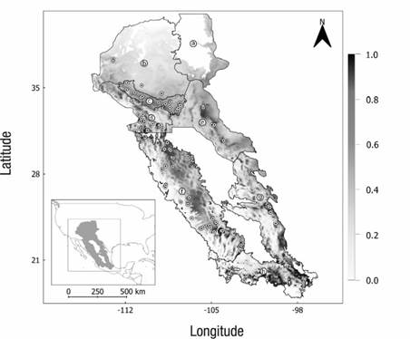
Figure 1 Historical potential distribution model (1970 to 2000) of the Mexican spotted owl (Strix occidentalis lucida): a) Southern Rocky Mountains, b) Colorado Plateau, c) Upper Gila Mountains, d) Basin and Range-West, e) Basin and Range-East in the USA, and f) Sierra Madre Occidental, g) Sierra Madre Oriental and h) Transverse Neovolcanic Belt in Mexico. Dots indicate occurrences (n = 155) of the Mexican spotted owl, used for model generation. The figure indicates discontinuous logistic prediction with darker areas (values close to 1) referring to those of higher bioclimatic suitability.
Bioclimatic predictors
The distribution of the Mexican spotted owl was most associated with the mean diurnal range of temperature (BIO 2), which contributed the most to the model prediction (44.8 %), the maximum temperature of the warmest month (BIO 5) was 28.8 % and the mean temperature of the coldest quarter (BIO 11) 19.5 %. The precipitation variables of the wettest month and quarter together only predicted 6.9 % of the model.
The response curves to the variables showed different bioclimatic thresholds for the Mexican spotted owl (Figure 2). The mean temperature range stabilized at a bioclimatic suitability of 11 °C and decreased dramatically with increasing temperature (up to 22 °C); the maximum temperature of the warmest month had the highest bioclimatic suitability at 17.5 °C; and the mean temperature of the coldest quarter stabilized at 5 °C, reflecting the environmental conditions of the mainly cold forests where the Mexican spotted owl inhabits. Bioclimatic suitability for precipitation ranged from 100-250 mm and 200-600 mm in the wettest month and quarter, respectively.
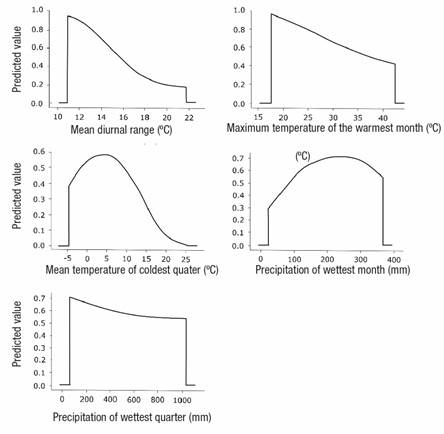
Figure 2 Response curves for each bioclimatic variable used as predictor in the potential distribution model of the Mexican spotted owl (Strix occidentalis lucida).
Jackknife analysis showed that the diurnal range of temperature (BIO 2) and maximum temperature of the warmest month (BIO 5) had the greatest regularized training gain (Figure 3). Precipitation of the wettest quarter (BIO 16) had the greatest gain when used in isolation containing useful information on bioclimatic conditions suitable for the subspecies. BIO 2 had the lowest decrease in gain when omitted and contained most of the information absent in the other variables to explain the bioclimatic niche of the Mexican spotted owl.
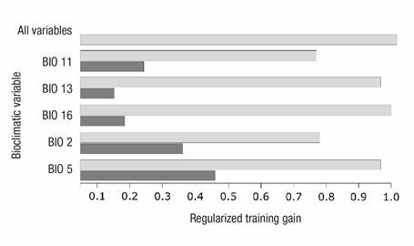
Figure 3 Regularized training gain for bioclimatic predictors of the Mexican spotted owl (Strix occidentalis lucida) distribution model using Jackknife analysis. Light gray bars represent regularized gain without a specific variable and dark gray bars represent regularized gain with only that variable. Bioclimatic variables: mean temperature range (BIO 2), maximum temperature of the warmest month (BIO 5), mean temperature of the coldest quarter (BIO 11), precipitation of the wettest month (BIO 13) and precipitation of the wettest quarter (BIO 16).
Future distribution
The distribution of the Mexican spotted owl varied spatially among climate change scenarios (Figure 4). Multidirectional movements and losses from 1.4 % to 96.4 % of suitable areas are predicted in all periods (Table 1). Although these losses vary among global climate models, the scenarios show a steady decrease in suitable bioclimatic space for the bird, especially in the EMU´s of Mexico. Models predicted gain of suitable bioclimatic areas for the Mexican spotted owl in the Southern Rocky Mountains, north of its historical distribution, being the only EMU that gained suitable bioclimatic space (51.3 to 167.2 %) in all periods.
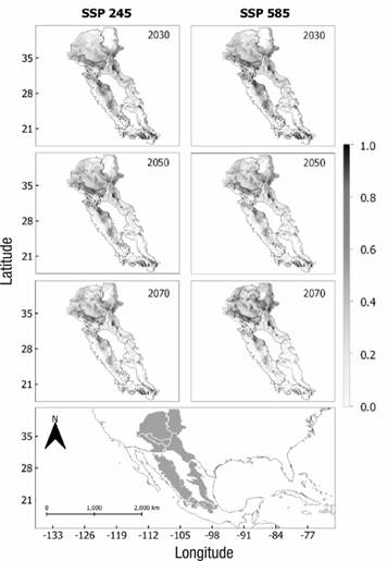
Figure 4 Potential distribution models for the Mexican spotted owl (Strix occidentalis lucida) for the periods 2021-2040 (2030), 2041-2060 (2050), 2061-2080 (2070) in ecological management units in the U.S. and Mexico, under two emissions scenarios (SSP). Images show logistic prediction with darker areas (values close to 1) indicating higher bioclimatic suitability.
Table 1 Variation in future bioclimatic space suitable for the Mexican spotted owl (Strix occidentalis lucida) in ecological management units in the United States and Mexico, considering low (SSP 245) and high (SSP 585) emissions climate change scenarios.
| Ecological management units | Historical distribution (km2) | SSP 245 | SSP 585 | ||||||
|---|---|---|---|---|---|---|---|---|---|
| Loss or gain (%) | Accumulation (km2) | Loss or gain (%) | Accumulation (km2) | ||||||
| 2030 | 2050 | 2070 | 2030 | 2050 | 2070 | ||||
| Southern Rocky Mountains | 4 783.10 | 59.7 | 68.3 | 90.9 | +4 347.8 | 51.3 | 102.3 | 167.2 | +7 997.3 |
| Colorado Plateau | 23 117.70 | -17.3 | -35 | -28.8 | -6 657.9 | -46.1 | -34.3 | -35.2 | -8 137.4 |
| Upper Gila Mountains | 5 351.40 | -1.4 | -2.9 | -8.4 | -449.5 | -2.1 | -7 | -8.7 | -465.6 |
| Basin and Range-West | 6 575.20 | -4.2 | -21.1 | -43 | -2 827.3 | -17.2 | -47.3 | -49 | -3 221.8 |
| Basin and Range-East | 14 724.00 | -34.6 | -49.5 | -63.9 | -9 408.6 | -29 | -57.2 | -66.1 | -9 732.6 |
| Sierra Madre Occidental | 20 751.20 | -15.9 | -39.1 | -54.4 | -11 288.7 | -21.1 | -50.6 | -65 | -13 488.3 |
| Sierra Madre Oriental | 11 368.10 | -61.5 | -83.5 | -87.5 | -9 947.1 | -56.1 | -84.9 | -96.4 | -10 958.8 |
| Transversal Neovolcanic Belt | 9 071.40 | -38.1 | -51.9 | -55.7 | -5 052.8 | -38.2 | -55.9 | -75.3 | -6 830.8 |
Future scenarios: 2021-2040 (2030), 2041-2060 (2050) y 2061-2080 (2070).
Discussion
Government agencies assess the effects of climate change on the geographic range of sensitive species (SEMARNAT, 2010; USFWS, 2012); to do so, they use species distribution models, which contribute to conservation plans (Guisan et al., 2013). Although the exclusive use of bioclimatic variables could simplify the biogeographic patterns of the Mexican spotted owl (Dallas, Decker, & Hastings, 2017; Salazar-Borunda et al., 2021b), the predicted bioclimatic suitability areas coincide with the current distribution areas (Salazar-Borunda, Martínez-Guerrero, Tarango-Arámbula, López-Serrano, & Pereda-Solís, 2022; USFWS, 2012). In this regard, the areas of bioclimatic suitability most suitable for the bird's permanence are greater in the center of the East and West Ranges and Basins, and Upper Gila Mountains in the USA, and in the center of the Sierra Madre Occidental, west of the Sierra Madre Oriental and scattered over the Transverse Neovolcanic Belt in Mexico.
Bioclimatic tolerance
The predictive yield of the model was higher using all evaluation metrics, showing the bioclimatic requirements of the Mexican Spotted Owl. Response curves and Jackknife tests identified the most important bioclimatic variables, which define the potential distribution of the bird. This subspecies shows tolerance to temperatures >5 °C but decreases to a mean temperature of 22 °C during the warmest month and, although it tolerates varying levels of precipitation (Salazar-Borunda et al., 2021b), it prefers areas with 200 to 250 mm in the wettest month, suggesting a link between relatively low temperatures and precipitation. This behavior may be associated with intrinsic mechanisms of thermoregulation and energy costs (Ganey, Ward, Rawlinson, Kyle, & Jonnes, 2020) and is consistent with field studies (Palma-Cancino et al., 2014; Silva-Piña et al., 2018) and previous models (Ganey et al., 2020; Palma-Cancino et al., 2020; Salazar-Borunda et al., 2022) that associate this raptor with mature forests in the U.S. and Mexico.
Future distribution
Climate change will undoubtedly continue to affect the natural distribution of bird species (Huntley et al., 2006). This effect will likely vary with current conservation condition, location, and ecology (Møller, Fielder, & Berthold, 2006). In this study, models predicted changes in the distribution range of the Mexican spotted owl over time, which do not represent significant changes for current populations; however, the loss of areas of bioclimatic suitability begins in 2030 and increases in 2041 and, therefore, represents a threat. Models showed a reduction in Mexico's EMU´s, especially in the Sierra Madre Oriental. Despite this, the remaining areas of suitability are restricted to the areas of historical distribution.
Changes in climate that affect the areas of suitability for the Mexican spotted owl and its survival have to do with physiology (Ganey et al., 2020), fecundity, abundance, and composition of prey communities (Franklin, Anderson, Gutierrez, & Burnham, 2000). These changes may modify the structure and composition of the mixed conifer forests in which the bird is naturally distributed (Gutiérrez & Trejo, 2014).
The results may be useful for monitoring and conservation of Mexican spotted owl populations; however, this study used few records of the subspecies (n = 155), so it is likely that this sample size compromised the accuracy of the model (Sagarin & Gaines, 2002; Salazar-Borunda et al., 2021b). The potential distribution of the Mexican spotted owl, generated in this study, is a first approximation that shows drastic effects of climate change on the suitable areas for this species in all the EMU´s. In this research, only five bioclimatic variables were used; however, in future studies, to obtain greater accuracy in prediction, these distribution models should also consider more specific variables such as topographic (Meineri & Hylander, 2017), vegetation (Pearson & Dawson, 2003), biotic interactions with prey (Wisz et al., 2013), potential competitors (Strix varia; Peterson & Robins, 2003) or human pressures (Engler et al., 2017). It will also be necessary to increase the number of records and project the model to larger geographic areas.
Conclusion
This study represents the first effort to define the effect of climate change on the potential distribution of the Mexican Spotted Owl. Predictive models of historical and future potential distribution, under two climate change scenarios, describe a gradual and steady decrease in areas of bioclimatic suitability for the bird and show new, more suitable bioclimatic sites north of its historical distribution, for example, in the Southern Rocky Mountains. Although losses of potential distribution areas for the Mexican spotted owl are accentuated after 2041, it is clear that climate change is already a threat to this bird of prey. In this study, only bioclimatic variables were used; therefore, future studies should include more specific variables such as topography, vegetation, biotic interactions with prey, potential competitors, and the effect of anthropogenic activities.

