


 texto em
  Inglês (pdf)
 Artigo em XML
 Referências do artigo
 Enviar este artigo por email
 Citado por SciELO
  Similares em
SciELO
Similares em
SciELO 
 Permalink
Highlights:
Aboveground biomass was estimated for medium-stature semi-evergreen and semi-deciduous tropical forests.
Aboveground biomass was estimated by applying the random Forest algorithm.
Spatial variation of precipitation and temperature are relevant for estimation and mapping.
The lowest uncertainty values were recorded for the semi-evergreen tropical forest.
Synergy of diverse data and automated algorithms provided biomass mapping.
Introduction
Tropical forests represent 45 % of the Earth's forest area and have high carbon storage capacity (Food and Agriculture Organization of the United Nations [FAO], 2020; FAO & UNEP, 2020). Unfortunately, in recent decades, these ecosystems have recorded high rates of deforestation and degradation (FAO, 2020) becoming sources of carbon dioxide into the atmosphere. Therefore, monitoring biomass (carbon) inventories and changes in the area of these forests is important for the planning of policies that contribute to the mitigation of negative effects of climate change (Dupuy-Rada, Hernández-Stefanoni, Hernández-Juárez, Tun-Dzul, & May-Pat, 2012; Houghton, Byers, & Nassikas, 2015).
Biomass can be monitored by collecting field data on a large number of sampling units, which represents a heavy investment in time and cost (Wulder et al., 2012); however, as relationships between field-measured biomass density and data from different types of remote sensors have been identified, it has been possible to reduce the number of field samples without sacrificing accuracy (Saatchi et al., 2011).
Information on vegetation type and conditions is provided by indices estimated from spectral values of satellite images (Foody et al., 2001). NDVI (normalized difference vegetation index) and SAVI (soil-adjusted vegetation index) have been the most widely used for modeling aboveground biomass, quantification of tree structure and composition of tropical forests (Foody et al., 2001; Ghosh & Behera, 2018). Other indices (brightness, greenness and wetness) estimated by Tasseled Cap transformation are able to distinguish phenological changes and key attributes in different forest types and conditions (Deo et al., 2016). LiDAR (Light Detection And Ranging) active sensors are considered a suitable technology for the study of forest structure, as they provide detail and spatial accuracy. LiDAR-derived metrics tend to be highly correlated with aboveground biomass measurements; therefore, methodologies that take advantage of this relationship are more beneficial when incorporating satellite image products, which cover the study area perfectly and provide information in areas of difficult access (Wulder et al., 2012).
LiDAR technology has restrictions of use for monitoring large areas, due to its high cost and the large amount of data for storage and processing. The viable option is to obtain data in strategically established stripes and rely on satellite image data to estimate variables of interest at a regional scale (Saatchi et al., 2011; Wilkes et al., 2015); furthermore, it is known that the lowest biomass estimation errors are achieved when using LiDAR-derived data and auxiliary variables from optical images and radar data (Zolkos, Goetz, & Dubayah, 2013). Accuracy of estimates depends on factors such as landscape heterogeneity, density of sampled data, and the remote sensors used. Hence the importance of estimating and expressing, spatially, the uncertainty of estimates at the pixel level (Barbosa, Broadbent, & Bitencourt, 2014).
Based on the above, this study aimed to identify a combination of spectral and climate variables to estimate aboveground biomass for two types of medium-stature tropical forest in the Yucatan Peninsula; to evaluate the behavior of the models fitted with the random Forest algorithm; and to map the aboveground biomass and its associated uncertainty at the pixel level. Estimates of aboveground biomass and its associated uncertainty, expressed spatially, can contribute to the management of policies to mitigate the effects of climate change in tropical forests.
Materials and Methods
Study area
The study area includes the medium-stature semi-deciduous (SMSC) and semi-evergreen (SMSP) tropical forests of the Yucatan Peninsula, Mexico (Figure 1). It covers approximately 77 000 km2, where 28 000 km2 correspond to SMSC and 49 000 km2 to SMSP (Instituto Nacional de Estadística y Geografía [INEGI], 2013).
SMSC has a warm sub-humid (Aw1) climate with rain in summer (May-October) and a dry season (November-April). Mean annual temperature is 26 °C (Dupuy-Rada et al., 2012). SMSP has a warm sub-humid climate with mean annual precipitation of 950 mm (July-October) and mean annual temperature of 22 °C (Aryal, De Jong, Ochoa-Gaona, Esparza-Olguin, & Mendoza-Vega, 2014). In most of the Yucatan peninsula, precipitation gradient is dry to the northwest (600 mm) and wetter to the southeast (1 400 mm) (Martínez & Galindo, 2002).

Figure 1 Study area: Medium-stature semi-deciduous and semi-evergreen tropical forests-series V, INEGI, 2013- of the Yucatan Peninsula, Mexico. Red stripes indicate the location of biomass data estimated from LiDAR data (Ortiz-Reyes et al., 2019).
Aboveground biomass data
This study used aboveground biomass estimates reported by Ortiz-Reyes et al. (2019), corresponding to raster files. These authors employed an area-based approach for biomass estimation by linking field measurements (data from the Inventario Nacional Forestal y de Suelos de México, 2009-2014 remeasurement) with LiDAR metrics, using the random Forest algorithm. Estimates from such protocol, frequently, maintain and even exceed operational accuracy standards than those obtained through traditional inventory, with an acceptable level of bias (White et al., 2013). Each pixel (20 m x 20 m) containing an estimated aboveground biomass value about the stripes were considered as “LiDAR plots”. These estimates increase the distribution and sample size of local data and are similar to field plot estimates (Wulder et al., 2012). Subsequently, the strip pixels were resampled to a spatial resolution of 30 m using the nearest neighbor method to match pixels from Landsat images (Cracknell, 1998).
Landsat images and climate data
Six Landsat 8 images taken by the OLI (Operational Land Imager) sensor, processed at the surface reflectance level (Vermote, Justice, Clavarie, & Franch, 2016) were downloaded from the United States Geological Survey database (USGS, 2017).
The image search period was one year (April 1, 2013 up to April 30, 2014) to establish closeness between the conditions of previous aboveground biomass estimates from LiDAR data with Landsat images. Those images with cloudiness less than 21 %, corresponding to the winter season, were downloaded (Table 1). A cloud mask was applied to each scene using the Pixel QA (Quality Assessment) filter (Vermote et al., 2016). The procedure was performed with the QGIS software version 3.6 Noosa (QGIS, 2019), using CloudMasking plugin. Cloud and shadow areas were excluded from subsequent analyses.
Table 1 Characteristics of Landsat 8 scenes processed at the ground reflectance level for the estimation of aboveground biomass for medium-stature tropical forests of the Yucatan Peninsula.
| Landsat scene identifier | WRS Path | WRS Row | Scene cloud cover (%) | Acquisition date |
|---|---|---|---|---|
| LC80190452014046LGN01SR | 19 | 45 | 2.08 | February 15, 2014 |
| LC80190462014046LGN01SR | 19 | 46 | 1.97 | February 15, 2014 |
| LC80190472014046LGN01SR | 19 | 47 | 10.79 | February 15, 2014 |
| LC80200452014005LGN01SR | 20 | 45 | 0.54 | January 5, 2014 |
| LC80200462014021LGN01SR | 20 | 46 | 8.3 | January 21, 2014 |
| LC80200472014005LGN01SR | 20 | 47 | 20.9 | January 5, 2014 |
Later, NDVI, MSAVI (modified soil-adjusted vegetation index), SAVI and EVI (enhanced vegetation index) spectral indices were created with the preprocessed images. Brightness, greenness and wetness indices were estimated using the Tasseled Cap transformation to take advantage of information from more bands, using coefficients for Landsat products with surface reflectance reported by Crist (1985). The above was estimated using the raster package in R (R Development Core Team, 2013). Spectral bands alone (2 to 7) were also used as independent variables in the estimation of aboveground biomass.
Climate information was taken from the WorldClim (2017) database which has monthly average, minimum and maximum temperature, and precipitation for the period 1970 to 2000. Average monthly temperature and monthly precipitation data were downloaded for January, February, November, and December, in addition to mean annual temperature (°C) and annual precipitation (mm), biologically significant variables (Fick & Hijmans, 2017). All these variables had ~1 km2 resolution so they were resampled to 30 m, using the nearest neighbor method, to match them with the other variables. These variables were chosen because of their proven relevance in other forest parameter estimation studies (Ahmed, Franklin, Wulder, & White, 2015; Wilkes et al., 2015). The list of predictor variables processed is shown in Table 2.
Table 2 Predictor variables (spectral and climate variables) used for modeling of aboveground biomass. Variables correspond to raster files.
| Variable (abbreviation) | Features/Formula | Trait |
|---|---|---|
| Band 2(B2fc) | B2 blue (λ: 0.452 - 0.512 μm) | Differentiates vegetation soil and deciduous coniferous vegetation (USGS, 2019) |
| Band 3(B3fc) | B3 green (λ: 0.533 - 0.590 μm) | Evaluates plant vigor (USGS, 2019) |
| Band 4(B4fc) | B4 red (λ: 0.636 - 0.673 μm) | Discriminates vegetation slopes (USGS, 2019) |
| Band 5(B5fc) | B5 Near infrared (λ: 0.851 - 0.879 μm) | Emphasizes moisture conditions of plants and soils (Young et al., 2017) |
| Band 6(B6fc) | B6 Shortwave infrared 1 (λ: 1.566 - 1.651 μm) | Emphasizes moisture conditions of plants and soils (Young et al., 2017) |
| Band 7(B7fc) | B7 Shortwave infrared 2 (λ: 2.107 - 2.294 μm) | Enhances soil and vegetation moisture content (USGS, 2019) |
| NDVI(bNDVIfc) |
|
Sensitive to photosynthetic activity (Ghosh & Behera, 2018) |
| MSAVI(bMSAVIfc) |
|
Sensitive to the amount of vegetation (Qi et al., 1994) |
| SAVI (bSAVIfc) |
|
Highly correlated with vegetation cover dynamics (Gao, Huete, Ni, & Miura, 2000) |
| EVI(bEVIfc) |
|
Sensitive to canopy structural variations (Gao et al., 2000; Vieilledent et al., 2016) |
| TCB(brighVal) |
|
Sensitive to ground brightness (Crist, 1985) |
| TCG(GreenVal) |
|
Sensitive to greenness of vegetation (Crist, 1985) |
| TCW (WetVal) |
|
Sensitive to moisture content of vegetation (Crist, 1985) |
| Mean annual temperature (Var_Bio1) | Data from 1970 to 2000 °C at 30” spatial resolution (~1 km2) | Influence vegetation growth and mortality processes (Álvarez-Dávila et al., 2017) |
| Annual precipitation (Var_Bio12) | Data from 1970 to 2000 mm at 30” spatial resolution (~1 km2) | Positive relationship with biomass. Influence vegetation growth and mortality processes (Álvarez-Dávila et al., 2017) |
| Average temperature for January (TemAv_M01), February (TemAv_M02), November (TemAv_M11) and December (TemAv_M12) °C | °C at 30” spatial resolution (~1 km2) | Influence activation of growth processes in plants (Fick & Hijmans, 2017) |
| Average precipitation for January (Prec_M01), February (Prec_M02), November (Prec_M11) and December (Prec_M12) | mm at 30” spatial resolution (~1 km2) | Influence activation of growth processes in plants (Fick & Hijmans, 2017). |
NDVI: normalized difference vegetation index; SAVI: soil adjusted vegetation index; MSAVI: modified soil adjusted vegetation index; EVI: enhanced vegetation index; TCB: Tasseled Cap brightness, TCG: Tasseled Cap greenness, TCW: Tasseled Cap wetness.
Aboveground biomass estimate using the random Forest algorithm.
From aboveground biomass data previously estimated by Ortiz-Reyes et al. (2019) in transects with LiDAR data (more than 300 000 pixels for each vegetation type), a sample of 5 000 pixels per vegetation type was randomly selected without replacement to fit two models and estimate the biomass for the entire area of interest. The sample of 5 000 pixels represented the values of the dependent variable (aboveground biomass). Climate data and spectral data recorded in Landsat images, corresponding to the same pixels of the random sample, represented the independent variables.
The random Forest algorithm of R (R Development Core Team, 2013) builds a set of decision trees from training data, which are internally validated to generate a prediction of the response variable given the predictors (Cutler, Cutler, & Stevens, 2012). The algorithm is easy to apply and capable of processing large databases efficiently, as an option in regional studies (Asner & Mascaro, 2014). Final predictor variables were selected regarding the influence that each one represented on the mean squared error (MSE) of the fitted model. Sequentially, the algorithm evaluated the performance of the model for each vegetation type based on RMSE (root mean square error), number of predictor variables and percentage of variance explained.
Mapping aboveground biomass in two types of tropical forest
Aboveground biomass maps were created in the R raster package (R Development Core Team, 2013). The maps were produced with the previously generated model using the raster files corresponding to the spectral and climate variables chosen by the model as relevant for predicting aboveground biomass.
Quantification of uncertainty
Uncertainty refers to the level of ignorance of the true value of a parameter or variable of interest due to multiple factors and can be quantified with common statistical estimators such as standard deviation, coefficient of variation (CV) or by an interval with a preset confidence level (Global Observation of Forest and Land Cover Dynamics [GOFC-GOLD]). This study evaluated and mapped uncertainty of aboveground biomass predictions by CV associated with the estimates generated at the pixel level. Estimataions were performed using the ModelMap package of R (Freeman, Frescino, & Moisen, 2018).
Results and Discussion
Models for estimating aboveground biomass in two tropical forest types
A separate model was fitted to estimate aboveground biomass in each medium-stature tropical forest type using the random Forest algorithm. The main parameters are shown in Table 3.
Table 3 Relevant parameters of the random Forest models for aboveground biomass estimation per type of medium-stature tropical forest in the Yucatan Peninsula.
| Parameters | Semi-evergreen tropical forest | Semi-deciduous tropical forest |
|---|---|---|
| R2 | 0.5 | 0.5 |
| r | 0.71 | 0.7 |
| RMSE (Mg·ha-1) | 34.1 | 26.2 |
| Number of predictor variables | 12 | 15 |
R2: coefficient of determination, r: correlation between measured vs. predicted aboveground biomass data, RMSE: root mean squared error.
Predictive ability of models is within the range reported in other studies for tropical forests (R2 = 0.50-0.92). Those studies used similar data and approaches to this research; for example, Lu et al. (2012) estimated aboveground biomass in the Amazon basin using a multiple regression model and differentiated mature (R2 = 0.50) and secondary successional (R2 = 0.76) forests. The authors point out that aboveground biomass estimation using Landsat images is site-dependent, due to variation in phenology, vegetation type and structure. In contrast, Basuki, Skidmore, Hussin, and Van Duren (2013) used images taken by a synthetic aperture radar (SAR) and Landsat ETM+ imagery for aboveground biomass estimation in tropical forests under management in Indonesia. By regression models, these authors explained 75 % of the variance (RMSE = 78.9 Mg∙ha-1), while in a tropical forest in Malaysia, Phua et al. (2017) attributed 63 % of the variance to LiDAR metrics and 18 % to Landsat 8 green band texture variables (RMSE = 112.15 Mg∙ha-1). Meanwhile, Ghosh and Behera (2018) estimated the aboveground biomass of two species grown in a tropical forest in India with SAR data and Sentinel-2A imagery; the explained variance was 60 % and 71 % (RMSE = 79.45 Mg·ha-1; 105.02 Mg·ha-1) with random Forest and Gradient Boosting autonomous learning techniques, respectively. At the regional scale, Asner and Mascaro (2014) estimated aboveground carbon density in 14 tropical ecoregions in five countries and, by fitting nonlinear maximum likelihood models, explained 92.3 % of the variance (RMSE = 17.12 Mg C·ha-1).
In the previous cases, prediction method yield was superior to that obtained in this study; however, the errors obtained were also high (RMSE between 78.9 Mg·ha-1 and 112.15 Mg·ha-1) compared to those of this study (RMSE = 34.1 Mg·ha-1 and 26.2 Mg·ha-1 for SMSP and SMSC, respectively). However, if results are compared with the regional study of Asner and Mascaro (2014), the reported error is similar in terms of aboveground biomass.
Regarding the variables selected by the random Forest algorithm (Figure 2), results showed that the green band (B3fc) and annual precipitation (Var_Bio12) were the most important in models for estimating aboveground biomass in SMSP and SMSC, respectively. Climate variables prevailed in predicting aboveground biomass in both medium-stature tropical forest types, pointing to an influence of climatic processes on estimated aboveground biomass. This influence has been recognized in several studies on biomass estimation in tropical vegetation (Álvarez-Dávila et al., 2017; Vieilledent et al., 2016).
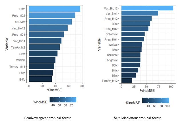
Figure 2 Relative importance of variables selected by the random Forest model in the medium-stature semi-evergreen tropical forest (12 variables) and the medium-stature semi-deciduous tropical forest (15 variables), for the estimation of aboveground biomass. B3fc: reflectance of Band 3 - green from Landsat 8 OLI sensor, Prec_M02: precipitation month 2 (February) (mm); bNDVIfc: normalized difference vegetation index; Var_Bio12: annual precipitation (mm); Prec_M01: precipitation month 1 (January, mm); Var_Bio1: mean annual temperature (°C); TemAv_M2: mean temperature of month 02 (February, °C); B2fc: reflectance of Band 2 - blue from Landsat 8 OLI sensor; WetVal: wetness in Tasseled Cap transformation; TemAv_M11: mean temperature of month 11 (November, °C); B6fc: reflectance of Band 6 - shortwave infrared 1 from Landsat 8 OLI sensor; B4fc: reflectance of Band 4 - red from Landsat 8 OLI sensor; Prec_M12: precipitation of month 12 (December, mm); GreenVal: greenness in the Tasseled Cap transform; B5fc: reflectance of Band 5 - near infrared from Landsat 8 OLI sensor; brighVal: brightness in Tasseled Cap transform; B7fc: reflectance of Band 7 - shortwave infrared 2 from Landsat 8 OLI sensor; TeamAv_12: average temperature of month 12 (December, °C). IncMSE %: percent increase in mean square error.
Regarding precipitation, the main constraint of dry forests is water in the soil, which could suggest relevance of annual precipitation (Var_Bio12) in the SMSC model, while monthly precipitation averages (Prec_M01, Prec_M02) remained in the modeling of both vegetation types. Cao et al. (2015) mention that the growth of this forest type not only varies with age, soil type or land use background, but also with precipitation.
The fact that precipitation and temperature remained as relevant variables in the models could be an indication of the relationship between amount of available water and its interaction with temperature to influence biomass growth processes. In such a case, both precipitation and temperature would be having superior control over aboveground biomass density in tropical forests, because both vary regionally and are scale-dependent (Álvarez-Dávila et al., 2017; White & Hood, 2004). Saatchi et al. (2011) report that spatial variability of aboveground biomass depends on climate, natural and human-induced disturbance and recovery processes, soil type and variations in topography. Martínez and Galindo (2002) mentioned that high spatial and temporal variability of precipitation, geological substrate and scarce development of the soil were decisive factors in the distribution of vegetation in an area with similar characteristics to the one evaluated in this study.
For biomass prediction in the SMSC, the random Forest algorithm selected the same or similar spectral variables that have shown good predictive capacity in forests with similar conditions. Freitas, Mello, and Cruz (2005) report that NDVI is a good indicator of aboveground biomass for dry and deciduous tropical forests. Of the spectral indices, NDVI was the only one that was maintained for both models, the rest of the indices were removed because they did not contribute to the yield of models. The blue, green and infrared bands were similar components to those reported in the study of Foody et al. (2001), who indicate the importance of regarding all useful sensor bands and not only the indices dependent on the red band. The green, red and infrared bands were maintained as explanatory variables in both vegetation types, highlighting the green band (B3fc). Such relevance was also reported by Foody et al. (2001) and Phua et al. (2017).
Mapping aboveground biomass for two types of medium-stature tropical forest
Figure 3 shows the spatial variation of aboveground biomass in the two types of medium-stature tropical forest. SMSP biomass ranged from 4.0 to 185.7 Mg·ha-1 (mean [ȳ] = 85.2; standard deviation [s] = 23.2), an interval that is within the results reported by other authors for the same type of vegetation. Aryal et al. (2014) reported values from 11.72 to 99.56 Mg C·ha-1 for four-year-old secondary forests (s = 4.92) and for mature forests (s = 20.83), which is similar to the interval reported in this study. Recently, Hernández-Stefanoni et al. (2020) reported 127.5 Mg·ha-1 of average aboveground biomass and a CV lower than 40 %.
For SMSC, aboveground biomass ranged from 11.7 to 117 Mg·ha-1 (ȳ = 51.1; s = 17.5). This value is within the range reported by Dupuy-Rada et al. (2012) for dry tropical forests of the Yucatan Peninsula (ȳ = 56 Mg·ha-1). Similarity could be due to the fact that aboveground biomass data of the two studies come from mosaics of forest fragments at different successional ages and spatial arrangement. For this vegetation type, Hernández-Stefanoni et al. (2020) reported 100.4 Mg·ha-1average aboveground biomass and Dai et al. (2014) estimated 5.0 to 115.0 Mg C∙ha-1 with ȳ = 56.6 Mg C∙ha-1.
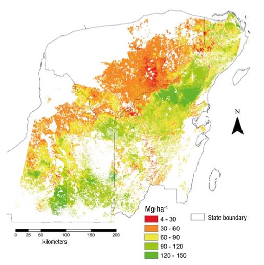
Figure 3 Spatial distribution of average aboveground biomass (Mg·ha-1) in medium-stature semi-evergreen and semi-deciduous tropical forests of the Yucatan Peninsula, Mexico
On the other hand, there are estimates that report higher amounts of aboveground biomass than that reported in the present study; e.g., Hernández-Stefanoni et al. (2014) reported mean biomass values of 109.71 Mg·ha-1 and 376.77 Mg·ha-1 for SMSC and SMSP, respectively, when they used field sampling plots of 1 000 m2. These same authors reported mean biomass values of 147.2 and 270.2 Mg·ha-1 for SMSC and SMSP, respectively, when using 400 m2 field sampling plots in the same study area. This shows the complexity of comparing results between studies of similar purpose, but using different methods or analysis approaches, specially when the size of the areas under analysis is uneven and landscape elements are contrasting as a result of spatially haphazard successional states due to anthropogenic activities and natural disturbances (Aryal et al., 2014; Dupuy-Rada et al., 2012).
Spatial uncertainty of aboveground biomass predictions
Spatial variability of prediction uncertainty was expressed as the percentage of CV (Figure 4). For SMSP, the CV ranged mostly between 25 and 75 % and was of higher magnitude for SMSC (75 to more than 100 %), particularly in areas with low average aboveground biomass and adjacent to others where information was removed, due to the hiding process to exclude cells containing clouds. These CV values, in general, are higher than those reported by Hernández-Stefanoni et al. (2020) for the same vegetation types (0 to 75 %, but mostly below 60 %); however, it is important to highlight the contrast in the size of the area analyzed in both studies. The aforementioned authors analyzed 3 600 km2 of each vegetation type, while in this study 28 000 km2 of SMSC and 49 000 km2 of SMSP were analyzed, therefore, it is to be expected that variability is greater.
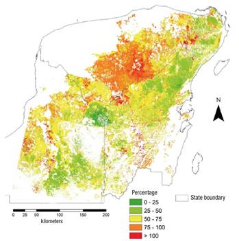
Figure 4 Spatial distribution of uncertainty (% coefficient of variation) of aboveground biomass in the medium-stature semi-evergreen and semi-deciduous tropical forests of the Yucatan Peninsula, Mexico.
Like most of the scarce research, this study used the CV to report spatial variation of uncertainty in biomass estimation. This highlights the importance of assessing uncertainty per component to identify which component contributes the most error to estimates. For example, two components that probably affected the results of this study are temporal discordance between field and remote sensing data, and the lack of a priori spatial planning of remote sensing data collection. Another component responsible for measured uncertainty is the model previously fitted by Ortiz-Reyes et al. (2019) to estimate aboveground biomass in stripes, whose data were used in this study as a starting point to fit a larger model by the random Forest algorithm. Therefore, the use of approaches that correct for the errors that each component adds is a pending task that could improve the precision of aboveground biomass estimates.
The analysis performed provides a record of the current biomass quantification effort and offers points of comparison on the road to improving uncertainty quantification methodologies in complex forest ecosystems. On the other hand, results represent an attempt to standardize the reports of spatial variation of uncertainty as an important part of forest aboveground biomass estimation.
Conclusions
Structural variability of medium-stature semi-deciduous (SMSC) and semi-evergreen (SMSP) tropical forests of the Yucatan Peninsula was collected by training data from stripes, which impacted the performance of models for predicting aboveground biomass in both vegetation types. Models provided a continuous map detailing spatial distribution of aboveground biomass at the pixel level for SMSC and SMSP. This distribution was explained in greater proportion by precipitation and temperature. The error of predictions, expressed as the coefficient of variation, allowed spatially explicit visualization of uncertainty associated with aboveground biomass estimation at 30 m resolution. Both the methodology and the results of this study are acceptable regarding the available elements and represent a contribution towards the development of more effective methods for estimating aboveground biomass at the regional level.

