


 texto en
  Inglés (pdf)
 Artículo en XML
 Referencias del artículo
 Enviar artículo por email
 Citado por SciELO
  Similares en
SciELO
Similares en
SciELO 
 Permalink
Introduction
Plant communities are distributed along the landscape depending on the gradients of various environmental factors (Pottier et al., 2013). Depending on the values of environmental factors, their significance, study area location, and structure and floristic composition of plant communities, species abundance can differ significantly (John et al., 2007; Vargot, Khapugin, & Chugunov, 2016; Lennon, Beale, Reid, Kent, & Pakeman, 2011; Popov & Makukha, 2019). Climatic and edaphic conditions of a habitat are often recognized as the strongest factors influencing the vegetation cover in a certain area (Dubuis et al., 2013; Gebremedihin, Birhane, Tadesse, & Gbrewahid, 2018; Khan, Khan, Ahmad, Ahmad, & Page, 2016; Pajunen, Kaarlejärvi, Forbes, & Virtanen, 2010). At the same time, the influence of climatic factors on vegetation is most noticeable at the regional or global scales (Jarema, Samson, McGill, & Humphries, 2009), while edaphic and topographic properties play a critical role in plant distribution at the local scale (Cui, Zhai, Dong, Chen, & Liu, 2009; John et al., 2007; Potts, Ashton, Kaufman, & Plotkin, 2002; Seregin, 2014).
Being based on environmental and phytogeographical gradients, most vegetation classifications are operated at various ecological scales (Landolt et al., 2010; Ramenskiy, Tsatsenkin, Chijikov, & Antipin, 1956; Tsyganov, 1983). Gradients associated with small-scale landscape heterogeneity, light availability and soil properties (pH, moisture, nitrogen availability) are well suited for the local scale. Nevertheless, climatic gradients and differences in the histories of local floras are also important at the regional or global level (Smirnova, Lugovaya, & Prokazina, 2013).
Ecological scales include plant species, which are responsive to changes in habitat conditions. Due to this fact, these plants act as phytoindicators that integrate many environmental factors. This is a very appropriate tool for understanding the environmental conditions of a habitat (e. g., climatic, edaphic, light conditions) when direct measurements are difficult (Gusev, 2009; Khapugin, 2017). Plant species can be used to indicate environmental conditions of habitats based on presence and/or abundance in the site (Goebel et al., 2001). The set of plant species contributes to distinguishing and mapping the conditions of landscape ecosystems based on the phytoindication approach. This could be especially important for searching for new locations for threatened plants, which have a narrower range of environmental conditions. In addition, in the study region (Republic of Mordovia) many of these species are Critically Endangered (e. g., Najas tenuissima [A. Braun ex Magnus] Magnus, Corallorhiza trifida Châtel., Huperzia selago [L.] Bernh. ex Schrank & Mart.) or Endangered (e. g., Cypripedium calceolus L., Pyrola media Sw., Scheuchzeria palustris L.) (Khapugin et al., 2017). Populations of some of them have not been re-discovered for a long time (e. g., Neotinea ustulata [L.] R. M. Bateman, Pridgeon & M. W. Chase - since 1888, Dactylorhiza viridis [L.] R. M. Bateman, Pridgeon & M. W. Chase - since 1980, Pedicularis dasystachys Schrenk - since 1985).
There are many studies devoted to distinguishing and characterizing the forest ecosystems (Goebel et al., 2001; Khan et al., 2016; Konollová & Chytrý, 2004; Priputina, Zubkova, Shanin, Smirnov, & Komarov, 2014) and/or succession processes (Budzáková, Galvanek, Littera, & Sibik, 2013; Khapugin et al., 2016; Priputina, Zubkova, & Komarov, 2015) in them in relation to different environmental factors. Fewer studies have been devoted to the mapping of the distribution of ecological factor gradients in forest systems (Bednova, 2014).
In this study, the approach of visualizing environmental factor gradients is presented for a certain area in the southern boundary of the taiga zone - within the Mordovia State Nature Reserve (Central Russia). The objective of this study was to determine an opportunity to identify suitable habitats for searched-for plant species based on phytoindication data.
Materials and methods
Study site
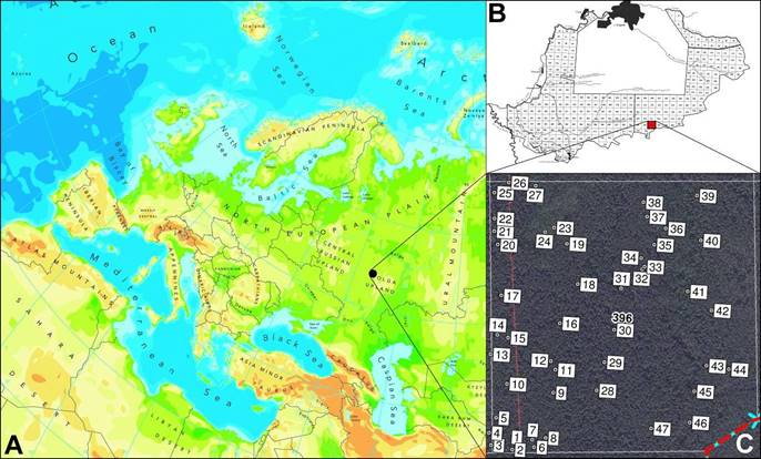
The study was carried out in the Mordovia State Nature Reserve (Figure 1), situated at the southern boundary of the taiga zone (54° 42' - 54° 56' N; 43° 04' - 43° 36' E; up to 190 m) in Central Russia. Total area of the Mordovia Reserve is 321.62 km2. Soils are classified as predominantly sand in varying degrees of podzolization. These lie on ancient alluvial sands (Kuznetsov, 2014). The mean annual precipitation in this area varies from 406.6 to 681.3 mm and the mean annual air temperature is 4.7 °C. Maximal temperature values are recorded in July, and minimal ones in February (Bayanov, 2015). Forest communities cover 89.3 % of the total reserve area. Pine (Pinus sylvestris L.) is the main forest-forming wood species. Birch (Betula pendula Roth) ranks second in the area covered by forest in the reserve. Lime (Tilia cordata Mill.) forests are encountered in the northern part of the reserve, whereas oak (Quercus robur L.) forests cover a relatively small area in the western section. Spruce (Picea abies L.) forests are located predominantly in the floodplains of rivers and streams and cover small areas (Tereshkin & Tereshkina, 2006).
Field sampling
The selected forest compartment (No. 396) is located in the south of the Mordovia State Nature Reserve. The Protected Area covers an area of 1.17 km2. This particular forest compartment was selected because: (1) the forest road, being evidence of human activity, passes through it from south to north; (2) it contains the oligotrophic bog in the northwest of the study area. In June 2017, 47 100-m2 square plots were randomly established within this area (Figure 1). Among them, three plots (45, 46, 47) were 2 × 50 m in size. They were established along the forest road. In each plot, plant species composition was recorded for further analysis. According to a vegetation map of the reserve, P. sylvestris is the predominant forest-forming species, with other trees being B. pendula and T. cordata.
Data analysis and visualization
To find the mean values (in scores) of the environmental factors in each plot, the Tsyganov (1983) ecological scale was used because it was specifically developed for the coniferous-deciduous forest subzone where the reserve is situated. Each environmental factor of the scale is represented by scores (gradations) depending on plant survival. It means that for a certain plant species the range of its existence in relation to a certain factor (for instance, soil nitrogen, moisture, etc.) can be identified. Since the study was carried out at the local scale, the edaphic and topographic environmental factors of the Tsyganov scale (1983) were selected: shading (LC), soil moisture (HD), soil nitrogen (NT), and soil pH (RC). The mean value of an environmental factor per each study plot was calculated as a mean of the entire set of species recorded there. It was calculated according to the following formula:
where,
mEFV |
mean environmental factor values (e. g., shading) |
|
the minimal score value of a factor in the Tsyganov scale (1983) for a plant species |
|
the maximal score value of a factor in the Tsyganov scale (1983) for a plant species |
n |
number of plant species in the floristical list in a study plot |
The distribution visualization of selected environmental factor gradients was performed using the relevant contour maps as background images using “Surfer” v. 11 software (Golden Software Inc., 2012). Interpolated contour maps were obtained by kriging using a default linear variogram. Calculated mean values of each environmental factor were used as the variables Z.
To reveal differences between plant species compositions in different study
plots, Jaccard’s similarity index
Statistical analysis was performed in MS Excel and PAST 3.15 (Hammer, Harper, & Ryan, 2001). The ordination techniques, the principal component analysis (PCA), were used to define the major gradients in the spatial arrangement of study plots of the analyzed dataset. For ecological interpretation of the ordination axes, mean values (in scores) of environmental factors for established plots were plotted onto a PCA ordination diagram as supplementary environmental data.
Results
Based on the calculated mean values of the environmental factors (shading, soil moisture, soil nitrogen, and soil pH) in each study plot, contour maps of selected environmental factor gradients were prepared. Figure 2 shows notable differences between the east and west parts of the selected forest compartment regarding all environmental factors. In addition, three study plots established along the forest road have not influenced the whole distribution of environmental factor gradients.
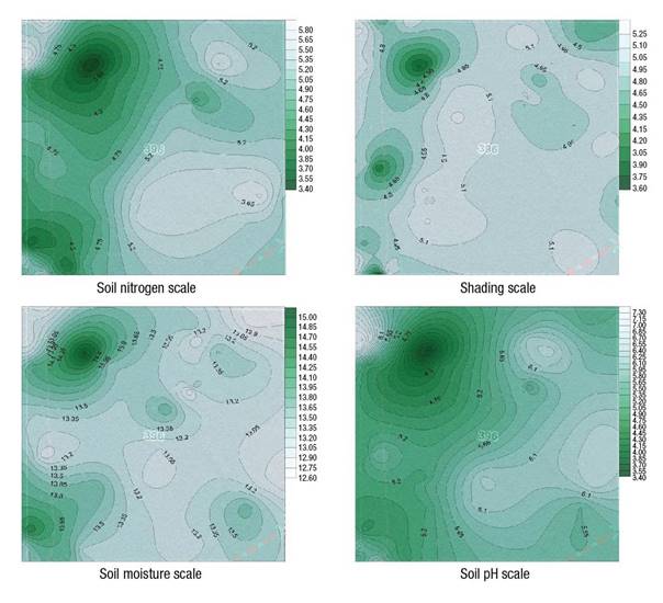
Figure 2 Interpolated spatial distribution maps showing the gradients of four selected environmental factors in the Mordovia State Nature Reserve.
Four spatial distribution maps of selected environmental factor gradients were combined with a decline in the layers’ visibility until 45 %-level. Hence, areas of the greatest overlap of all obtained maps were produced (Figure 3A). Then this map was combined with the scheme of the study plots within the selected forest compartment (Figure 1). As a result, three groups of study plots were obtained (Figure 3B). They are characterized by using maps from Figure 2. First group: the darkest area contains the most illuminated and moistest study plots with extremely low levels of soil pH and soil nitrogen. Forest communities present other distinguishable groups. Second group: the lightest area in Figure 3 is located predominantly in the eastern part of the forest compartment with three loci in its central-western, northwestern and southwestern parts. These areas are covered by moderately shaded forest communities on the most nitrogen-rich and alkaline soils. Third group: light-gray to dark-gray areas indicate the most shaded plant communities located on moderately acidic soils with a low level of soil nitrogen. It should be noted that soil moisture did not differ significantly between the first and second groups.

Figure 3 The combination of four maps showing the distribution of mean environmental factor values (A) and the same in combination with the map of study plots in the selected forest compartment (B) of the Mordovia State Nature Reserve.
In order to test and demonstrate more clearly this definition of study plots divided into three groups, PCA was performed on the values of four environmental factors for all study plots. All study plots have been arranged mainly along gradients of three soil parameters, namely pH, nitrogen availability and moisture (Figure 4), while habitat shading has not acted as strongly to the arrangement of most study plots. However, it is suggested that habitat shading and soil moisture should be considered as important factors determining vegetation structure formation in wider areas if these will include more various habitat types.

Figure 4 Principal component analysis (PCA) ordination diagram of plots established in the selected forest compartment of the Mordovia State Nature Reserve. Symbols: red triangles - group 1, blue squares - group 2, green dots - group 3. Environmental factors: LC = shading, HD = soil moisture, NT = soil nitrogen, RC = soil pH. To reveal ecological gradients, mean values of environmental factors were plotted onto PCA ordination diagram as supplementary environmental variables.
Ecological scales are based on plant species composition in a certain area. In the present study, each study plot was considered as such area. It was assumed that the use of any similarity indices should indicate the same distinguishing of study plots as demonstrated in Figure 4. In order to test that, plant species compositions of all study plots were compared using Jaccard’s similarity index.
A list was compiled of the plant species recorded in all study plots within the selected forest compartment. According to Khapugin and Astashkina (2018), there were 101 species of vascular plants from 43 families and four bryophytes in this area. Based on this list, Jaccard’s similarity indices were calculated. Obtained results are presented using cluster analysis (Figure 5). They show separation of all study plots into four main clusters. Of these, three clusters correspond to three groups of areas distinguished in Figure 3 and Figure 4, while the fourth cluster includes study plots situated along the forest road. It is noteworthy that no one map of environmental factor gradients reflected the location of the forest road based on phytoindicators from three study plots (Figure 2).
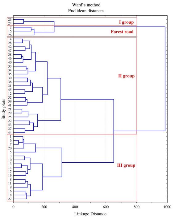
Figure 5 Cluster analysis dendrogram of plant species composition of 47 study plots in the selected forest compartment of the Mordovia State Nature Reserve, based on Jaccard’s similarity indices.
As can be seen, most study plots of the “afforested” second and third groups are arranged into two individual clusters. Three study plots (2, 15, 26) distinguished earlier into group 2 were placed in the separate cluster being combined with plots of group 1. These three study plots were established along the forest road containing several ruderal and grassland species. The combination of group 1 and the “forest road” group is a result of the lower similarity of their species composition with the species composition of the other two groups of study plots. Moreover, Jaccard’s similarity indices between study plots of group 1 and the “forest road” plots are equal to null.
Discussion
Gradient maps obtained of four selected environmental factors in the selected forest compartment demonstrated remarkable similarity. This suggestion is confirmed by the distinguishing of three areas because of overlapping of these maps. These areas are characterized by unique compositions of plant species. It is obvious that exactly these plant species determine most differences between three areas distinguished in Figure 3. Table 1 shows the lists of species unique to each distinguished group taking into account the “forest road” species forming a separate cluster in the dendrogram of Figure 5. Despite eight species recorded only along the forest road (plots 2, 15, 26), it did not affect the distribution of the gradients of selected environmental factors in the plant community (Figure 2). Obviously, the influence of these ruderal and meadow plants (Alchemilla vulgaris L., Persicaria hydropiper [L.] Delarbre, Plantago major L., Poa annua L.) on the gradients of selected environmental factors has been smoothed due to the dominance of species typical of the forest system (Convallaria majalis L., Asarum europaeum L., Molinia caerulea [L.] Moench, Sorbus aucuparia L.). Therefore, their influence on environmental factors in the study area can be considered as minimal.
Table 1 List of species unique to each group distinguished based on phytoindication data in the selected forest compartment of the Mordovia State Nature Reserve.
| Groups of uniqueness (percents) | Plant species |
|---|---|
| Species unique to group I (50.0 %) | Betula pubescens Ehrh., Carex lasiocarpa Ehrh.RC, Eriophorum vaginatum L.NT, LC, Ledum palustre L.NT, LC, Sphagnum fallax H. Klinggr.HD, Vaccinium uliginosum L. |
| Species unique to group II (57.4 %) | Acer platanoides L., Aegopodium podagraria L.NT, RC, *Alchemilla vulgaris L.NT, LC, Alnus glutinosa (L.) Gaertn., Angelica sylvestris L.HD, LC, Antennaria dioica (L.) Gaertn.HD, LC, Anthoxanthum odoratum L.RC, LC, Asarum europaeum L.HD, NT, RC, Athyrium filix-femina (L.) RothNT, LC, Carex elongata L.HD, NT, RC, *Carex leporina L.NT, Carex pallescens L.NT, RC, Chimaphila umbellata (L.) Nutt.HD, RC, Corylus avellana L., Daphne mezereum L.HD, LC, Epilobium angustifolium L., Equisetum sylvaticum L.HD, NT, *Festuca pratensis Huds.NT, LC, Galium mollugo L., Glechoma hederacea L.LC, Gymnocarpium dryopteris (L.) NewmanHD, RC, Hieracium sylvularum Jord. ex BoreauHD, Hieracium umbellatum L.NT, RC, Juniperus communis L., Lathyrus vernus (L.) Bernh.HD, Lonicera xylosteum L.HD, Melampyrum nemorosum L.HD, NT, RC, Mercurialis perennis L.HD, NT, Orthilia secunda (L.) HouseHD, NT, Paris quadrifolia L.HD, NT, Pilosella officinarum Vaill., *Plantago major L.LC, Platanthera bifolia (L.) Rich.HD, LC, *Poa annua L.NT, LC, Poa nemoralis L., Poa pratensis L.LC, *Persicaria hydropiper (L.) DelarbreLC, *Prunella vulgaris L., Pulmonaria obscura Dumort.HD, NT, RC, Pyrola rotundifolia L.HD, Ribes nigrum L., *Rumex acetosella L.NT, RC, LC, Salix caprea L., Sambucus racemosa L.HD, Scirpus sylvaticus L.RC, Scrophularia nodosa L., Silene viscaria (L.) Jess.NT, Stellaria graminea L., Stellaria media (L.) Vill., Veronica chamaedrys L., Veronica officinalis L., Viburnum opulus L.NT, Vicia sylvatica L.HD, RC, Viola rupestris F. W. SchmidtHD, NT, RC |
| Species unique to group III (19.1 %) | Calluna vulgaris (L.) HullNT, RC, Carex brunnescens (Pers.) Poir.HD, Carex globularis L.HD, LC, Carex vesicaria L.RC, LC, Dryopteris cristata (L.) A. GrayRC, Juncus conglomeratus L.RC, LC, Linnaea borealis L.NT, RC, Lycopodium clavatum L.NT, RC, Sphagnum girgensohnii Russow. |
Numbers in brackets are proportions of unique species of all species in a group; species unique only to the forest road (Figure 5) are marked by an asterisk (*). Superscripts designate specialist species relative to a certain factor: HD = soil moisture, RC = soil pH, NT = soil nitrogen, LC = habitat shading.
At the same time, there is a problem in determining the locations of ruderal (occasional here) species using the method presented here. The important question is, can a location of a certain species be revealed using gradient maps of selected environmental factors? It can be said that it is partially possible. So, survival intervals of the Tsyganov (1983) ecological scale can be used to separate all species into specialists (species with narrow intervals) and generalists (species with wide intervals) (Begon, Townsend, & Harper, 2005; Komarov & Zubkova, 2012). As specialists live in narrow limits of environmental factors, it is possible to reduce the search area for a certain plant, having gradient maps of environmental factors and the list of specialist species presumably living here. For instance, all maps obtained in the present study have demonstrated a strong difference in the area in the northwestern part of the forest compartment (Figures 2 and 3). According to phytoindication data (Figures 2 and 4), this is the most illuminated and moistest area on poor-nitrogen and acidic soils that corresponded to oligotrophic bogs of Eurasia (Wheeler & Proctor, 2000). Such environmental conditions were revealed in the northwestern part of the study area containing plots of group 1. Indeed, the oligotrophic Sphagnum-Eriophorum-dominated bog (Vargot, Khapugin, Chugunov, & Grishutkin, 2016) is located there where Vaccinium uliginosum L., Carex lasiocarpa Ehrh., Eriophorum vaginatum L., and Ledum palustre L. were recorded being specialist species in relation to certain environmental factors.
Practical benefits of environmental factor gradient visualization relate to forest system management and nature conservation tasks. The first benefit concerns an opportunity to establish the basic relations of selected environmental factors in a study area. It is especially important because understory plant species are considered as a sustainable indicator tool (Abella & Shelburne, 2004; Host & Pregitzer, 1991), generally retaining these properties after violation or destruction of an ecosystem (Khapugin et al., 2016; Sterk et al., 2016). Thus, the data received using the presented methodology will remain relevant for a long time.
The second benefit relates to the forecasting possibility of the locations for specialist plants (i. e. plants with narrow survival intervals) in a forest ecosystem. As shown above, a habitat with extreme environmental conditions could be identified based on phytoindication data and knowledge of the coenotical preferences of a species. Predicting suitable habitats of threatened (in particular locally rare [Crain & White, 2011]) plants is a high priority for biodiversity conservation tasks, especially since these species show on average significantly narrower habitat preferences in comparison with common species (Wamelink, Goedhart, & Frissel, 2014). For instance, Daphne mezereum L. has been included in the additional list of the Red Data Book of the Republic of Mordovia (Silaeva, 2017). In the Mordovia State Nature Reserve this species is known in the undergrowth layer of deciduous and mixed forests (Vargot et al., 2016), i.e. it inhabits forests with relatively high soil pH and nitrogen availability. Based on Figure 3, D. mezereum is more likely to be found in habitats defined in group 2, i.e. in both western and/or three small areas in the eastern parts of the selected forest compartment. Indeed, D. mezereum was found in study plots 22 and 42 (Figure 3). Thus, although it is not completely possible to indicate the concrete location of a plant, the search area can be limited. For instance, the search area for D. mezereum was limited to 58.1 % - from 1.17 km2 (full area of the forest compartment) to 0.68 km2 (area of the forest compartment related to group 2).
Finally, the third benefit of the presented methodology is an opportunity to use phytoindication data obtained from any ecological scale used in the world (Ellenberg, Weber, Düll, Wirth, & Werner, 2001; Landolt et al., 2010; Ramenskiy et al., 1956; Tsyganov, 1983). The main requirement is the need to identify the most suitable ecological scale for a certain study area.
Despite the benefits demonstrated in this case study, it should be noted that this methodology will be more accurate if more data on mean environmental factor values is obtained in a region. In addition, it is more suitable for specialist species which can grow in habitats with less variable environmental conditions or for narrowly-specialized groups of plants (aquatic habitats, oligotrophic wetlands, among others). The presented methodology is not able to reveal localities suitable for casual plant species (e. g., ruderal, alien plants) because they are unable to influence significant changes in the environmental conditions of an undisturbed habitat. Their presence could be determined only by using floristic similarity indices.
Conclusions
The use of phytoindication methods allows constructing maps of environmental factor gradients for a certain forest area. A map creation is not a new method but combined with species similarity indices it could be used for predicting habitat suitability for threatened plant species. It is especially important due to some threatened plants being able to lead an underground life under unfavorable conditions. Values of environmental factors can be used for map construction based on any existing ecological scales. First, the most appropriate ecological scale should be adequately determined for a certain study. Secondly, the fieldwork procedure should be accurately followed using an appropriate method depending on the selected ecological scale.

