


 texto en
  Inglés (pdf)
 Artículo en XML
 Referencias del artículo
 Enviar artículo por email
 Citado por SciELO
  Similares en
SciELO
Similares en
SciELO 
 Permalink
Introduction
According to the Forestry Institute (INFOR, 2016), the Chilean forestry industry produced 8.7 million m3 of sawn timber in 2015. In Chile, 1 270 sawmills currently operate; the number of units classified as small increased 12 % (<5 000 m3·month-1) and medium-sized units increased 2 % (5 000 to 10 000 m3·month-1) (INFOR, 2016). Sawmills transform logs into finished pieces by applying successive cuts. Raw material yield depends on how the logs are processed (Álvarez-Lazo, Andrade-Fernando, Quintín-Cuador, & Domínguez-Goizueta, 2004); according to Walker (2006), it is the main factor influencing operational performance and profitability. For Flores-Velázquez, Serrano-Gálvez, Palacio-Muñoz, and Chapela (2007), low-productivity sawmills have low-tech machinery and equipment, which makes them inefficient in converting raw materials. These plants have limited mechanization, process low-quality logs, are labor-intensive, and exhibit unbalanced production flows (Álvarez-Lazo et al., 2004; Flores-Velázquez et al., 2007).
Discrete event simulation (DES) allows designing load capacities and eliminating critical machines in various supply scenarios (Wolfsmayr, Merenda, Rauch, Longo, & Gronalt, 2016). On production lines, analysis has been performed using analytical and simulation models. The former exhibits unrealistic assumptions; for example, reliable machines, processing distribution, continuous feeding and no blockages in the machines, while, according to Heshmat, El-Sharief, and El-Sebaie (2013), simulation models allow the identification of flow restrictions and optimization for line redesign in a reliable way. DES has also been used in value stream mapping in order to find improvement opportunities without the need to alter the system under study (Parthanadee & Buddhakulsomsiri, 2014). Simulation allows mimicking a process and analyzing configurations without the need to intervene in it (Meimban, Mendoza, Araman, & Luppold, 1991; Quintero & Rosso, 2001).
DES has been applied in forest harvest planning and its logistics (Di Gironimo et al., 2015; Hogg, Pulkki, & Ackerman, 2010; Marques, De Souza, Rӧnnqvist, & Jafe, 2014; Memari, Zahraee, Anjomanshoae, & Rahim, 2013; Spinelli, Di Gironimo, Esposito, & Magagnotti, 2014). In particular, there is research focused on location decisions, size of temporary storage stations (Meimban et al., 1991), equipment evaluation, production flow and critical machines (Baesler, Araya, Ramis, & Sepúlveda, 2004; Grigolato, Bietresato, Asson, & Cavalli, 2011; Opacic & Sowlati, 2017; Opacic, Sowlati, & Mobini, 2018). DES is implemented in programs based on structured programming language to formulate models in any application area (Heshmat et al., 2013); however, it has not yet been applied to study worker-machine behavior nor has it been extensively combined with optimization (Opacic & Sowlati, 2017).
Optimization is used in the development of forest production plans, although these do not explicitly consider stochastic factors (Lohmander, 2007). By combining optimization and DES, dynamic events can be anticipated, producing realistic and useful solutions for decision support systems (Marques et al., 2014). In this sense, Azadeh and Maghsoudi (2010) and Baesler et al. (2004) verified the results delivered by the DES model by applying the t-test, integrated them with experimental design (ED) by defining decision factors (k-factors) and evaluated the effects on the response variable using factorial experiments.
Quintero and Rosso (2001), Baesler et al. (2004) and Grigolato et al. (2011) used DES and developed flow studies in bulk-cut sawmills. In such studies, homogeneous-grade logs were sorted by diameter and processed in batches, applying a predetermined cutting plan. These authors applied DES to explore flow restrictions and through ED evaluated equipment substitution and plant and raw material distribution scenarios, allowing for increased flow and productivity in the sawmill process.
In the case study of custom-cut sawmills, heterogeneous-grade logs are processed individually without diameter sorting. Therefore, a flexible cutting plan is applied to each log depending on its grade and size, the appearance of the piece obtained and the production order. In this scenario, flow analysis considers the dynamic adjustment of machines and transports, which is complex to address with analytical approaches (Meimban et al., 1991). So far, only Thoews, Maness, and Ristea (2008) have studied, in part, the case of bulk and custom sawing in various wood species using DES and ED. Therefore, the objective of this research was to optimize the production flow in a high-production, custom-cut sawmill that processes Pinus radiata D. Don logs without diameter sorting (1 489 to 1 663 logs per shift) using DES and ED.
Materials and methods
The study was carried out in a custom-cut sawmill that processes P. radiata logs with diameters between 33 cm and 44 cm, whose sawn timber production line has a capacity of 180 000 m3 per year. The industrial plant is located in the city of Los Angeles, VIII Region of Biobío, Chile.
Sawmilling process
The sawmill's production flow began with the debarking process (Figure 1), which is intended to protect the cutting tools in the later sawing. Each log was then processed on two bandsaws with carriage. To do this, the log was positioned and fixed on the carriage’s moving squares, and the carriage advanced facing the bandsaw where cuts were sequentially made according to the diameter and quality of the log (primary cuts). The pieces in process, resulting from the primary cuts, were transported and processed in two double horizontal resaw bandsaws (bandsaw 1 and bandsaw 2), obtaining sawnwood pieces with a defined thickness. The pieces requiring an additional process were sent to a single horizontal resaw bandsaw (bandsaw 3). The next step was to eliminate the edges present on the borders of each piece, which also involved dimensioning their width. The operation was performed by three circular edgers (edger 1, edger 2 and edger 3). Finally, the pieces were transported to a board separating machine, where they were sorted for separator placement and final packaging.

Logic of cutting decisions
The cutting plan is a logical sequence of successive cuts, defined by the operation of bandsaws with carriage. Figure 2 illustrates the three cutting decisions based on log diameter.

1.. Diameter less than or equal to 34 cm. For this case, the log was sawn in two parts by the main machine, requiring a single cut.
2.. Diameter between 36 and 42 cm. The log was sawn in four parts, requiring three cuts.
3.. Diameter greater than or equal to 44 cm. The log was sawn in five parts, requiring four cuts.
When making cuts on the bandsaw carriage, processing times varied according to log diameter and length, as well as the number of pieces delivered to the next machines. Thus, the routes taken by the pieces depend on the number of units queued in the transports of the following machines and the capacity of units queued in the transport between the machines involved. When the capacity is exceeded, the transports and machines are stopped or blocked, which can occur forward or backward from the production flow.
Development and validation of the simulation model
The sawmill has a series of transports and cutting machines that are operated in a synchronized manner by the equipment operators according to the type and quantity of pieces in process. The process presents failures in machines, variability in diameters and number of pieces that trigger high randomness. These attributes prevent its analysis with static models based on time studies. Therefore, in this research, a DES model was developed to analyze critical machines and evaluate opportunities for improvement.
The DES model was developed based on the logic of the cutting decisions for each log diameter. This logic was incorporated into the programming of the DES model through "virtual" labels that identified the entities (logs, pieces in process and finished pieces) advancing in the process. This identification allowed determining, for each entity, the cutting decision, the number of pieces to be obtained, and the direction of the production flow based on the processing capacity of the transports and machines in relation to time. The behavior of each machine in the system was examined and the flow of pieces was analyzed based on the cuts applied to the processed logs, under the different production scenarios. The DES requires that the characteristic times of the production process be treated with their variability; therefore, they must be transformed into probability distributions. The processing, failure and arrival times of entities (logs, pieces in process and finished pieces) at each workstation were recorded, and probability distributions were fitted for each of them. Based on historical information, two simulation models were developed for sawing P. radiata logs with lengths of 2.5 and 5.0 m, and diameters between 34 and 44 cm. This raw material was sawn to produce sawnwood at a single thickness of 5/4" with variable width. The number of logs processed per shift was considered as the model’s response variable. The logic of cutting decisions and the processing times of the equipment were programmed and entered into the Arena® 3.5 discrete event simulation software package (Arena, 2007).
Critical machines and possible alternative flows were identified and their impact on the production flow was determined with a factorial experiment (k factors). The simulation model was validated by comparing the sawmill’s actual production indicators against those obtained by the simulation model. In particular, the number of logs processed per shift and the production per shift were compared, concluding that the DES model is a good representation of the actual system. Subsequently, the production flow study was initiated. For this, the simulation model was iterated and performance results of the machines and transports were obtained. The appropriate number of samples for analysis was obtained with a pilot test of five iterations of the model, with the purpose of obtaining the preliminary descriptive statistics of the process. The next step was to determine the number of model iterations according to a desired error and confidence level. Therefore, the number of replications or iterations to be performed, for each production flow study scenario in the model, was calculated using the formula suggested by Montgomery, Runger, and Medal (1996):
where,
n |
number of model replication for the desired level of accuracy |
S x |
standard deviation of the sample |
|
mean of the pilot runs |
t α/2, n-1 |
critical value associated with the t-Student distribution |
p |
precision level using error (α) of 5 % (p = 1-α) |
In this way, a number of 10 replicates was obtained for each production scenario (two log lengths) with an extension of 480 min for each run of the model, equivalent to one production shift of the sawmill. To determine the base production condition or pattern of the sawmill, the production results with 2.5 m and 5.0 m long logs were subjected to a descriptive statistical analysis and Tukey’s multiple comparison test (P = 0.1).
Identification of critical machines
The results of the five iterations of the simulation model were analyzed by determining the number of processed logs, units queued in transports between machines, machine usage factor, machine failure factor, factor without machine feeding, and blocking factor of each machine. Consequently, workstations with a usage factor close to 100 % and their number of queued units close to their design capacity were identified as critical machines.
Application of the experimental design for the evaluation of the factors
A full 2k factorial experimental design was applied for the purpose of determining whether there is statistically significant evidence that the factors evaluated influenced the "production level" response variable. The factors identified and considered were:A) deliver from bandsaw carriage 1 to bandsaw 3; B) double debarker capacity; C) eliminate the failures of bandsaw 1 and 2; D) directly deliver the pieces from bandsaw 2 to edger 2 directly.
The effect of the factors was evaluated in the "applied" (+) and "not applied" (-) operational levels with respect to the reference condition, represented by the sawmill without making any type of change. Finally, the experimental design was evaluated with the Design Expert 6.0 statistical package (Design Expert, 2007).
Results and discussion
Identification of critical machines and proposals for improvement
The results at the production level for the base condition or pattern, represented by the current sawmill production flow, were: 1 489 logs per shift for 2.5 m long logs and 1 663 logs per shift for 5.0 m long ones (Table 1). Tukey's multiple comparison test showed statistically significant differences (P = 0.1) in production volume when processing different log lengths. This behavior is consistent with that recorded by authors such as Steele (1984) and Cown, McConchie, and Treolar (1984), who reported an increase in production and yield by increasing the diameter and length of processed logs. On the other hand, these values coincided with the actual production data recorded in the sawmill, which fully validated the results obtained with the iterations of the DES model.
Table 1 Production of Pinus radiata logs with lengths of 2.5 and 5.0 m.
| Log length (m) | Log production per shift | Volume of sawn timber per shift (m3)* |
|---|---|---|
| 1 489 ± 73.38 | 251 a | |
| 5.0 | 1 663 ± 77.35 | 418 b |
*Average production volume by indirect calculation. ± Standard deviation of the mean. Different letters denote means with statistically significant differences (Tukey’s test, P = 0.1).
Like Baesler et al. (2004) and Thoews et al. (2008), the results of the DES model were used to detect critical machines; although the detected machines differ, the same search method was applied focusing on machines that showed a high utilization rate. The results of the model with respect to the time use of the sawmill machines allowed identifying these machines and proposing modifications to the flow of semi-finished pieces. The modifications or factors evaluated are shown in Table 2.
Table 2 Analysis of critical machines and factors to be evaluated in a custom-cut sawmill processing Pinus radiata timber.
| Factor | Identified situation | Evaluated factor |
|---|---|---|
| 1 | High use rate of resaw bandsaw1 | Direct delivery from band carriage 1 to bandsaw 3. |
| 2 | Debarker with high use factor and following machines with a high percentage of non-feeding time. | Increased processing capacity of the debarker. |
| 3 | For 5 m long logs: edger 3 with high use factor that causes bottlenecks in the previous machine and bandsaw carriage 2. | Flow change. Direct delivery of pieces from bandsaw 2 to edger 2. |
| 4 | Bandsaws 1 and 2 with design problems in their output transport and with frequent failures that cause short interruptions. | Complete elimination of failures in bandsaws 1 and 2. |
Analysis of the proposed scenarios
The variety of factors to be studied can be very diverse; that is, from the increase in capacity of critical machines (Baesler et al., 2004) and the storage location and size of products in process (Heshmat et al., 2013), to changes in the distribution of the logs used in the sawmill (Grigolato et al., 2011). However, this research focused on the first two factors, given that the sawmill is supplied with logs on the open market, which cannot be controlled.
The model generated 16 treatments from four evaluated factors. Table 3 shows the results of the effect of individual and combined factors on the response variable (logs per shift) in each production scenario (log length).
Table 3 Effect of the factors evaluated in each production scenario (log length) in a custom-cut sawmill processing Pinus radiata timber.
| Response variable average (logs per shift) | ||||||
|---|---|---|---|---|---|---|
| Treatment | Factors | Log length (m) | ||||
| A | B | C | D | 2.5 | 5.0 | |
| 1/Control | - | - | - | - | 1 489 | 1 663 |
| 2 | + | - | - | - | 1 505 | 1 694 |
| 3 | - | + | - | - | 1 512 | 1 740 |
| 4 | + | + | - | - | 1 519 | 1 734 |
| 5 | + | - | + | - | 1 534 | 1 739 |
| 6 | + | + | + | - | 1 536 | 1 866 |
| 7 | + | - | - | + | 1 551 | 1 692 |
| 8 | + | + | - | + | 1 574 | 1 750 |
| 9 | - | - | + | - | 1 586 | 1 752 |
| 10 | + | - | + | + | 1 601 | 1 723 |
| 11 | - | - | - | + | 1 609 | 1 700 |
| 12 | - | + | + | - | 1 624 | 1 809 |
| 13 | + | + | + | + | 1 634 | 1 916 |
| 14 | - | - | + | + | 1 661 | 1 777 |
| 15 | - | + | - | + | 1 717 | 1 793 |
| 16 | - | + | + | + | 1 766 | 1 928 |
Factors: A) delivery from bandsaw carriage 1 to band saw 3; B) doubled debarker capacity; C) failures eliminated from bandsaw 1 and 2; D) pieces directly delivered from bandsaw 2 to edger 2. The effect of the factors was evaluated at the "applied" (+) and "not applied" (-) operational levels with respect to the reference condition.
Analysis of the model for 2.5 m long logs
The analysis of variance (ANOVA) showed that the model was significant (F = 15.38; P < 0.001), with only a 0.1 % probability that it could be affected by some factor not included (Table 4). Similarly, when observing the F value of each factor individually, it was found that factor D had a greater effect on production, followed by factors A, C and B. As a whole, the factors were able to predict 84.83 % of the sawmill's production; therefore, the proposed model was able to adequately explain the production of 2.5 m long logs.
Table 4 Analysis of variance for the production of 2.5 m long Pinus radiata logs.
| Source of variation | Sum of squares | Degrees of freedom | Mean squares | F value | Prob>F |
|---|---|---|---|---|---|
| Model | 82 876 | 5 | 16 576 | 15.38 | <0.001* |
| A | 16 256 | 1 | 16 256 | 12.80 | 0.004* |
| B | 7482 | 1 | 7 482 | 5.89 | 0.034* |
| C | 13 572 | 1 | 13 573 | 10.69 | 0.008* |
| D | 40 804 | 1 | 40 804 | 32.13 | <0.001* |
| Residual | 13 971 | 11 | 1 270 | ||
| Total corrected1 | 92 086 | 15 | |||
| Standard deviation | 30.35 | R2 | 0.8483 | ||
| Mean | 1 588.63 | Adjusted R2 | 0.7931 | ||
| Coefficient of variation (%) | 1.91 | Predicted R2 | 0.6790 | ||
| Sum of squared errors of prediction | 29 558 | Adequate accuracy2 | 13.364 |
*Significance level of 10 % by F test. 1Represents the sum of A + B + C + D + residual. 2Measures the model's signal-to-noise ratio; generally, a value above four indicates a strong signal and, therefore, a reliable model.
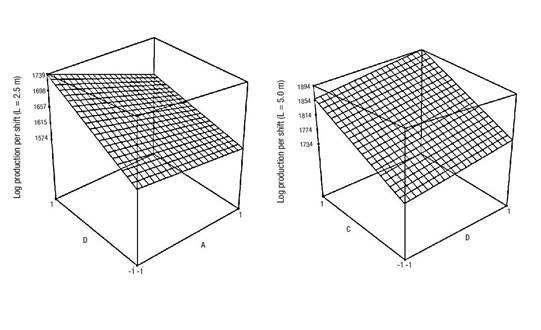
The response surface of the model allows visualizing the conditions under which the highest sawmill production is obtained (Figure 3), which is possible to attain by setting factors B, C and D at their maximum level (+) and factor A at its minimum level (-). This allows production to be increased by 13 % with respect to the initial condition, that is, the production level increased from 251 to 298 m3·shift-1 of finished product.
Analysis of model for 5.0 m long logs
ANOVA showed that the model was significant (F = 25.12, P < 0.001), with a 0.1 % probability that it could be affected by some factor not included (Table 5). Similarly, when observing the F value of each factor separately, factor B had a stronger influence on production and, in a lesser order, factors C and D. These factors together predict 86.26% of production; therefore, the model adequately explains sawmill production when processing 5.0 m logs.
Table 5 Analysis of variance when processing 5.0 m long Pinus radiata logs.
| Source of variation | Sum of squares | Degrees of freedom | Mean squares | F value | Prob>F |
|---|---|---|---|---|---|
| Model | 79 167 | 3 | 26 389 | 25.12 | <0.001* |
| B | 39 601 | 1 | 39 061 | 37.70 | <0.001* |
| C | 34 596 | 1 | 34 596 | 32.93 | <0.001* |
| D | 4 971 | 1 | 4 971 | 4.73 | 0.050* |
| Residual | 12 605 | 12 | 1 050 | ||
| Total corrected1 | 91 773 | 15 | |||
| Standard deviation | 32.41 | R2 | 0.862 | ||
| Mean | 1 767 | Adjusted R2 | 0.828 | ||
| Coefficient of variation (%) | 1.83 | Predicted R2 | 0.755 | ||
| Sum of squared errors of prediction | 22 410 | Adequate accuracy2 | 14.054 |
*Significance level of 10 % by F test. 1Represents the sum of A + B + C + D + residual. 2Measures the model's signal-to-noise ratio; generally, a value above four indicates a strong signal and, therefore, a reliable model.
The response surface of the model allowed us to visualize the desirable process conditions (Figure 3), which are obtained when factors B, C and D are set at their maximum level; in this way, production increases by 18 % with respect to current production, being equivalent to an increase from 418 to 475 m3·shift-1. In general, a large effect of factors B, C and D was observed when changing the length of the logs. Although the diameter distribution was not studied as a factor, the results showed an improved process flow when using 5.0 m long logs. This is probably due to the fact that the output transports of the machines are more efficient when processing longer than shorter pieces. It is therefore suggested that future research should study the effect of diameter distribution on productivity.
The applied methodology that analyzes the results obtained with a DES model, through a factorial experimental design, identified opportunities to increase production between 13 % and 18 % when 2.5 and 5.0 m long logs, respectively, are processed. These results are consistent with those obtained by Baesler et al. (2004), who report increases of between 6.3 % and 17.4 % in a bulk-cut sawmill, and are lower than the 31.5 % obtained by Thoews et al. (2008).
Generally, simulation research focuses only on identifying critical process machines to increase productivity; however, Heshmat et al. (2013) also addressed the design of transport capacity to keep pieces in process. This approach could be highly useful in redesigning the production flow of sawmills and it is suggested that it be addressed in future research.
Conclusions
The developed model enabled us to understand the dynamic flow of the process and identify the critical factors affecting it. The most sensitive factors impacting productivity were: factor B (increased debarker capacity), C (elimination of failures in the bandsaws when changing log length) and D (direct delivery from bandsaw 2 to edger 2). Low-mechanization sawmills with a minimum degree of engineering design show greater potential for improvement by employing the applied approach. Although the application of discrete event simulation is demanding in terms of time capture and programming, once developed it is easily reproducible. Therefore, the resources used in its application will drop drastically, making its application feasible in future research.

