


 texto en
  Inglés (pdf)
 Artículo en XML
 Referencias del artículo
 Enviar artículo por email
 Citado por SciELO
  Similares en
SciELO
Similares en
SciELO 
 Permalink
Introduction
In forestry research, there are several methods to characterize the structure and density of mixed-species and uneven-aged stands. The maximum density can occur after crowns closure is complete, but this is rarely observed because, generally, the canopy of a stand presents empty spaces; the proportion of these is greater as the trees grow. Therefore, the actual condition of density fluctuates around a level of equilibrium called normal density and can approach the maximum under unusual growth conditions, when most growth spaces are covered (Zeide, 2004).
Relative density functions or measures describe the degree of clumping of trees that form a stand or forest, in relation to a standard density condition (Torres-Rojo & Velázquez-Martínez, 2000). The most used in forestry research are based on the Reineke’s density index (Reineke, 1933), tree-area ratio (Chisman & Schumacher, 1940), relative space index (Wilson, 1946), crown competition factor (Krajicek, Brinkman, & Gingrich, 1961), Yoda’s density index Yoda, Tatuo, Husato, & Kazuo, 1963) and in the relative density index (Curtis, 1970, Drew & Flewelling, 1979). These measures were developed assuming specific conditions in the stands, such as the homogeneous composition of species and specific age distribution; however, it is difficult to find these characteristics in forests with forest management (Torres-Rojo & Velázquez-Martínez, 2000). The simplest measure of density is the number of trees per unit area, which is used successfully to quantify the density or competition in a growing space and the size of the trees in a stand (Burkhart, 2013).
During the growth and development of trees in a stand, intense competition for light, nutrients and growth space can induce mortality; this process is known as dense-dependent, mortality or self-thinning (Pretzsch, 2009, Yoda et al., 1963). The self-thinning “law” or rules of Reineke (Reineke, 1933) and Yoda (Yoda et al., 1963) assume a common slope between the logarithm of average tree size and the logarithm of the density or number of trees per unit of area (-1.605 for Reineke and -1.5 for Yoda), for mixed-species stands in the maximum density line (Burkhart, 2013).
The density-size relationship, maximum density and self-thinning have been modeled for even-aged stands and, occasionally, for uneven-aged stands. Some of the studies carried out are the following: Cao, Dean, and Baldwin (2000) described the changes between the mean square diameter and the density in stands with the presence of self-thinning of Pinus elliottii Engelm.; Torres-Rojo and Velázquez-Martínez (2000) created a model of relative density based on the Reineke’s density index for mixed-species stands; Bi, Wan, and Turvey (2000) estimated the upper line of the self-thinning for biomass and density of Pinus radiata D. Don with the econometric procedure known as the stochastic frontier function for even-aged stands; Long and Shaw (2005) generated a density management diagram for uneven-aged stands of Pinus ponderosa Douglas ex C. Lawson with forest inventory data; Comeau, White, Kerr, and Hale (2010) studied the maximum density relationship for Picea sitchensis (Bong.) Carr. and Pseudotsuga menziessii Mirb. Franco using density models for even-aged and continuous cover stands; García (2012) studied the principles of density "laws" or self-thinning rules and created density management diagrams for stands with and without thinning; Burkhart (2013) studied the behavior of diameter, height and volume to estimate the number of trees in self-thinning stands and the prediction of growth in stands with different age, density and site index; Reyes-Hernandez, Comeau, and Bokalo (2013) evaluated the density-size relationship in pure and mixed-species stands of Populus tremuloides Michx. and Picea glauca (Moench) Voss, with the stochastic frontier regression approach and indicated that the size-density relationship can satisfactorily developed for mixed-species stands; and Santiago-García et al. (2013) determined the self-thinning line in stands of Pinus patula Schiede & Cham. with the stochastic frontier regression methods and ordinary least squares, for the models of Reineke and Yoda, and concluded that the first method provides an efficient alternative to estimate the maximum density line.
A density management diagram is a graphical tool that relates the stand density and the average size of trees (volume, biomass, basal area or mean square diameter) per unit area (Drew & Flewelling, 1979). Site occupation is the most important property in mixed-species stands; when there is a mixture of species in a stand, the density management study should focus on all the species present and include the interspecific and intraspecific competition.
The objectives of this study were to compare the maximum density lines of mixed-species stands with the Reineke’s model, adjusted by ordinary least squares (OLS) and stochastic frontier regression (SFR); and create a density management diagram (DMD) to prescribe thinning in mixed-species stands for timber production purposes in the state of Durango, Mexico.
Materials and methods
Study area and experimental data
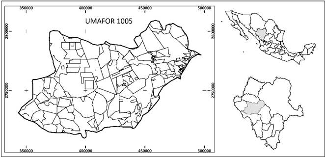
The data used in the fitting of density-size relationship (number of trees per hectare based on the mean square diameter) were obtained from mixed-species forest stands at the Forest Management Unit (UMAFOR) 1005 "Santiago Papasquiaro y Anexos" in Durango, Mexico (Figure 1). The study area is located in the northwest region of the state of Durango, between 24° 30’ - 25° 27’ N and 105° 01’ - 106° 24’ W. The total area of the UMAFOR 1005 is 859 496.59 ha, of which there are 639 936.77 ha of timber production, 120 014.95 ha of restoration, 32 510.60 ha of protection and 67 034.27 ha for other uses (agriculture, livestock and grassland). The predominant climates are cold temperate with cold summers and mean annual temperature between 5 and 12 °C, and subhumid temperate with mean annual temperature between 12 and 18 ° C. The warmest season is from May to June with maximum temperatures of 26 to 28 °C; the minimum temperatures vary from -4 to -6 °C in December and January (García, 1981).
A total of 1 760 circular plots from the forest inventory of 0.10 ha, distributed close to the maximum density line, were used for this study to fit the number of trees per hectare (N) and the mean square diameter (Dg) as a Reineke’s model (Reineke, 1933). Table 1 shows the descriptive statistics of the dataset for the adjustment of the density-size relationship (N-Dg) for mixed-species forests.
Table 1 Descriptive statistics of 1 760 plots from the mixed-species forest inventory of UMAFOR 1005 "Santiago Papasquiaro y Anexos" in Durango, Mexico.
| Variable | Mean | SD | Minimum | Maximum |
|---|---|---|---|---|
| G (m2·ha-1) | 28.00 | 8.38 | 4.27 | 65.31 |
| Vta (m3·ha-1) | 269.32 | 114.83 | 53.87 | 837.30 |
| Vtap (m3) | 0.79 | 0.62 | 0.07 | 4.09 |
| H0 (m) | 16.64 | 5.26 | 6.00 | 39.00 |
| D0 (cm) | 37.04 | 10.52 | 10.00 | 100.00 |
| A (years) | 102.65 | 27.63 | 27.00 | 290.00 |
| SI (m) | 22.81 | 8.19 | 10.00 | 35.00 |
| Dg (cm) | 29.74 | 8.45 | 12.60 | 56.57 |
| N (trees·ha-1) | 502.00 | 277.00 | 20.00 | 1 415.00 |
G = basal area, Vta = total volume of the tree, Vtap = total volume of the tree average per tree, H0 = dominant height, D0 = dominant diameter, A = average age, SI = site index of the dominant species of the genus Pinus, at a reference age of 60 years (the SI was estimated with the equation reported by , Dg = Mean square diameter, estimated as Dg = [(G/N)/(π/40000)]0.05, N = density and SD = standard deviation of the mean.
The dataset of inventory plots included the proportion of trees per species in relation to the total number of trees: Pinus durangensis Martínez (23.37 %), P. arizonica Engelmannii (8.40 %), P. leiophylla Schlecht. & Cham. (2.41 %), P. teocote Schlecht. & Cham. (12.85 %), P. engelmannii Carr. (0.76 %), P. lumholtzii B. L. Rob. & Fernald (0.91 %), P. ayacahuite Ehrenb. (10.45 %), P. herrerae Martínez (0.15 %), Quercus sideroxyla Humb. & Bonpl. (12.80 %), Q. durifolia Seem (11.01 %), Q. resinosa Liebm. (2.35 %), Q. crassifolia Ehrenb. (0.23 %), Q. rugosa Neé (1.60 %), Juniperus deppeana Steud. (3.76 %), Arbutus xalapensis Kunth (5.25 %) and P. menziessii (3.70 %). With respect to the global basal area, P. durangensis had the highest value (7.14 m2·ha-1) and, as for the spatial distribution, it was associated with Q. sideroxyla (6.88 m2·ha-1), P. arizonica (5.20 m2·ha-1) and P. teocote (4.33 m2·ha-1). The lowest value of the basal area was for A. xalapensis (1.29 m2·ha-1).
Statistical analysis
In the modeling of the density-size relationship, most studies discuss the empirical validation of the self-thinning law, where the presence of subjectivity in the selection of maximum density data has become the main point of analysis. Common methods for estimating the maximum density line have been based on the use of information from stands growing at that density. Therefore, the self-thinning line is modeled, before it occurs, as the average adjusted by OLS and the result is a maximum average in contrast to an absolute maximum, which technically should be the correct limit. This subjectivity implies that the same dataset can be analyzed to provide evidence of rejection or to draw different conclusions. The SFR method, as a production function, estimates the maximum density limit and more efficiently than OLS (Bi et al., 2000; Santiago-García et al., 2013) when the data come from temporary plots of forest inventory. This implies that all plots can be used to estimate the maximum density line (Reyes-Hernandez et al., 2013). In this study, the occupation property of the site was used to model the density of mixed-species stands, because all species represent the maximum occupation in a given condition and interspecific and intraspecific competition occur at the same time.
The Reineke’s model (Reineke, 1933) was used to establish the density-size relationship (N-Dg) of mixed-species stands. The model expresses the number of trees per hectare as a function of the mean square diameter (
where,
In |
natural logarithm |
N |
density (trees·ha-1) |
Dg |
mean square diameter (cm) |
β0 y β1 |
Intercept and the slope parameters of the maximum density line, respectively |
ɛi |
random error with the property |
The SFR method is considered a very efficient procedure to adjust the maximum density line when the data could present autocorrelation and heteroscedasticity (Reyes-Hernandez et al., 2013). The form and parameters of the Reineke’s model, which reflect growth mechanisms, can generate controversies in biological and statistical terms, but are very efficient to describe the functional relationship N-Dg (Zeide, 2005). In addition, the model constant is a measure of intraspecific competitive capacity called self-tolerance (Zeide, 1985). The Reineke’s model has been used to generate the maximum density line in pure (Cao et al., 2000) and mixed-species (Torres-Rojo & Velázquez-Martínez, 2000) forests. For SFR, the model is given by the log-log expression, such as the formulation of a Cobb-Douglas type model with two error terms (Aigner, Lovell, & Schmidt, 1977):
where
The stand density index (SDI) for the species mix is defined as the number of trees per hectare at a mean square diameter of reference (25 cm for this case). This conception applies to stands with any degree of density, because the slope parameter (
On the other hand, to estimate the number of trees per hectare as a function of SDI, the following expression is used:
The SDI per species and the SDI for the mixture of species is estimated with the following expressions, respectively:
where
The average growth space (S, m2) or available average area, for the mixture of species, was obtained with the expression S = (10 000 m2/
Model fitting
The adjustment of the model with OLS was performed in The MODEL Procedure of SAS/ETS® 9.3 with the Gauss-Newton optimization method; while the adjustment with SFR was made in The Q-LIM Procedure of SAS/ETS® 9.3 with the Quasi-Newton optimization method through maximum likelihood (Statistical Analysis System [SAS Institute Inc.], 2011). The SFR approach with superior statistical properties was selected through the following adjustment statistics: likelihood logarithm (LogLik), Akaike’s information criterion (AIC), Schwarz’s information criterion (SBC), total variance of the error component (σ) and variance ratio of the error components (λ).
Development of the density management diagram
The DMD was constructed with the equation obtained by SFR with N-T for the density-size relationship and using the maximum SDI (100 %) for mixed-species stands. DMD growth areas were defined according to the Langsaeter theory (Daniel, Helms, & Baker, 1979; Gilmore, O'Brien, & Hoganson, 2005; Langsaeter, 1941; Smith, Larson, Kelty, & Ashton, 1997). In this theory, the density management scenarios are defined, which implies maximizing the individual growth of residual trees (Santiago-García et al., 2013). The hypothesis establishes that the production of total volume in a stand, with specific age and composition, is constant and optimal for a range of point densities. The density may decrease, but not increase, with the modification of the forest inventory or point density (Gilmore et al., 2005; Langsaeter, 1941).
Due to the complexity of interspecific and intraspecific relationships of species, influence of species composition, stand characteristics and site factors, it is difficult to establish a general hypothesis for the definition of growth zones (del Río et al., 2015). In research on DMD for uneven-aged and mixed-species stands, Long and Shaw (2012) mention that the key to the design of the density management regime is the appropriate definition of the minimum and maximum limits of relative density. These researchers defined the upper limit at 60 % of the SDImax (550) and the lower limit at 35 % of the SDImax (220). According to this information, in this study, the line of imminent mortality or self-thinning was defined at 70 % of the SDImax and the lower limit at 35 % of the SDImax.
Results and discussion
For the line of maximum density obtained with OLS, the intercept and slope were statistically different from zero (P < 0.0001) (Table 2). However, this adjustment characterizes a central tendency line considered inadequate to describe the upper limit of the density-size relationship, because it tends to overestimate mortality.
Table 2 Parameter estimates of the Reineke’s model with the ordinary minimum square method for mixed-species forests.
| Parameter | Estimates | SE | t | Pr > t | LL | UL | MSE | RMSE | R2 adj |
|---|---|---|---|---|---|---|---|---|---|
|
|
12.274 | 0.085 | 143.29 | <0.0001 | 12.106 | 12.442 | 0.102 | 0.319 | 0.75 |
|
|
-1.860 | 0.025 | -73.06 | <0.0001 | -1.910 | -1.810 |
SE = parameters standard error; t = value of the Student's t distribution; Pr > t = value of the probability associated with the Student's t distribution; LL and UL = lower and upper limits of the 95 % confidence interval, respectively; MSE = Mean square error; RMSE = Root-mean- square error; and R2 adj = Adjusted coefficient of determination.
Table 3 shows the parameter estimates obtained by SFR for the approaches H-N, N-E and N-T, the components of the error variance of the stochastic production function and the statistical adjustment. The approach N-E was comparatively better than H-N and N-T, because it had the highest likelihood logarithm (LogLik = -411) and the lowest values of the Akaike’s information criterion (AIC = 830), Schwarz’s information criterion (SBC) = 851) and error variance (σ = 0.316); however, H-N and N-T were better adjusted to the upper boundary line of the experimental data (Figure 2).
Table 3 Parameter estimates of the Reineke’s model with the stochastic frontier regression (SFR) method, under different approaches, for mixed-species forests.
| Approach | Parameter | Estimates | SE | t | Pr > t | LogLik | AIC | SBC |
|
|
|---|---|---|---|---|---|---|---|---|---|---|
| H-N |
|
12.4021 | 0.0911 | 136.08 | <0.0001 | -424 | 856 | 877 | 0.472 | 2.494 |
|
|
-1.7953 | 0.0273 | -65.79 | <0.0001 | ||||||
|
|
0.1753 | 0.0097 | 18.04 | <0.0001 | ||||||
|
|
0.4376 | 0.0159 | 27.51 | <0.0001 | ||||||
| N-E |
|
12.1756 | 0.0884 | 137.71 | <0.0001 | -411 | 830 | 851 | 0.316 | 1.019 |
|
|
-1.7639 | 0.0268 | -65.71 | <0.0001 | ||||||
|
|
0.2217 | 0.0084 | 26.27 | <0.0001 | ||||||
|
|
0.2258 | 0.0131 | 17.20 | <0.0001 | ||||||
| N-T |
|
12.3534 | 0.1418 | 87.08 | <0.0001 | -958 | 1925 | 1953 | 0.484 | 0.782 |
|
|
-1.6602 | 0.0602 | -27.53 | <0.0001 | ||||||
|
|
0.3811 | 0.0543 | 7.02 | <0.0001 | ||||||
|
|
0.2982 | 0.0304 | 9.80 | <0.0001 | ||||||
|
|
0.4688 | 0.0372 | 12.59 | <0.0001 |
H-N, N-E and N-T = approaches of SFR half-normal, normal-exponential and normal-truncated, respectively; SE = parameters standard error; t = value of the Student's t distribution; Pr > t = value of the probability associated with the Student's; LogLik = likelihood logarithm; AIC = Akaike information criteria; SBC = Schwarz information criterion; σ = total variance of the error; λ = reason for the variances of the error components.
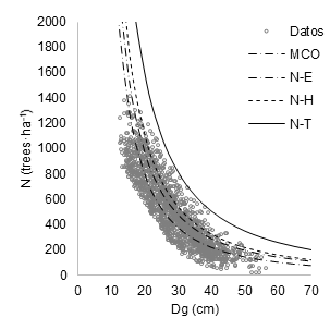
Figure 2 Maximum density lines for mixed-species stands, adjusted with ordinary least squares and stochastic frontier regression (SFR). The approaches of SFR are represented by H-N (half-normal), N-E (normal-exponential) and N-T (normal-truncated).
The 95 % confidence interval for the slope parameter, adjusted by SFR with NT N-T (-1.541 to -1.778), was wider compared to that adjusted by OLS (-1.810 to -1.910), SFR with H-N (-1.714) to -1.910) and SFR with N-E (-1.711 to -1.816). However, SFR with N-T adjusted the maximum density line to the upper limit of the data from the mixed stand plots. The 95 % confidence interval of the intercept parameter overlaps between the methods used; OLS (12.106 to 12.442), SFR with H-N (12.223 to 12.580), SFR with N-E (12.002 to 12.349) and SFR with N-T (12.075 to 12.631). The extreme values of the intercept for the mixture of species are contained in the lower limit of SFR with N-E and the upper limit of SFR with N-T.
The maximum density line created by SFR with the approach N-T showed better fit to the upper limit of the maximum density of the mixed stand data. Although it does not have the greatest adjustment (in this case the adjustment should not be a problem for the detection of the appropriate density threshold), this line was used to generate the DMD shown in Figure 2.
Density management diagram and thinning program
The DMD based on the adjustment of SFR as a N-T model is shown in Figure 3. The maximum density line represents the SDImax (1 107) at an mean square diameter of 25 cm; the line of imminent mortality or self-thinning was represented at 70 % of SDImax (775); the lower line of the constant growth area was defined at 35 % of the SDImax (387); and the free growth line at 20 % of the SDImax (221). These four lines defined the DMD growth zones: 1) free growth (20 % < SDImax ≤ 35 %), 2) constant growth (35 % < SDImax ≤ 70 %), 3) mortality (70 % < SDImax ≤ 100 %).
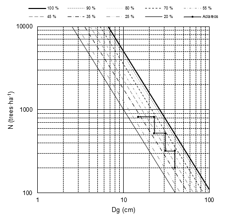
Figure 3 Density management diagram created by adjusting stochastic frontier regression (SFR) with normal-truncated approach (N-T) and thinning program for mixed-species stands.
The DMD includes different isolines with defined proportions within each growth area, as well as the effect of a thinning program for a mixed-species stand of the dataset. The thinning program is based on the initial condition of N = 820 trees·ha-1, Dg = 15 cm, G = 14.5 m2·ha-1 and SDI = 352. This stand contains the following species with their respective proportions and SDI: P. durangensis (47 %, 165), P. arizonica (22 %, 78), P. teocote (19 %, 67) and Q. sideroxyla (12 %, 42).
Thinning was programmed exclusively within the zone of constant growth (zone III), in which production is dense-independent and growth is maximized for residual trees. The first thinning is applied when the stand reaches the condition close to the line of imminent mortality with G = 31 m2·ha-1, Dg = 23 cm and SDI = 714. The conditions after thinning are N = 520 trees·ha-1, SDI = 453, Dg = 23 cm (a systematic thinning is applied and Dg should remain constant) and G = 12.5 m2·ha-1. Two thinning was carried out before reaching the final harvest. In the previous condition, the conditions are N = 200 trees·ha-1, Dg = 40 cm, G = 25.13 m2·ha-1 and SDI = 436; and in the final harvest, G = 36.13 m2·ha-1, Dg = 48 cm and SDI = 591 with the initial species proportion. The thinning program is applied in accordance with the 15-year cutting cycle and a 90-year forest rotation. The planning of the program depends on the objectives, either to maintain the species mixture or only one of these for the final harvest or to regularize the structure for the next forest rotation.
Figure 4 shows the graph of maximum density line (SDImax or 100 %) in three dimensions. The graph presents the number of trees per hectare (N) with respect to the mean square diameter (Dg) and the percentage of the basal area (G). For each combination of N and Dg, the percentages of the basal area belong to the same SDI. In the line of the reference square diameter (Dg = 25 cm), the standardized basal area is shown for each SDI. These SDI coincide directly with the SDI of 1 107 (100 %), 996 (90 %), 886 (80 %), 775 (70 %), 609 (55 %), 498 (45 %), 387 (35 %), 227 (25 %) and 221 (20 %), according to the DMD isolines (Figure 3).
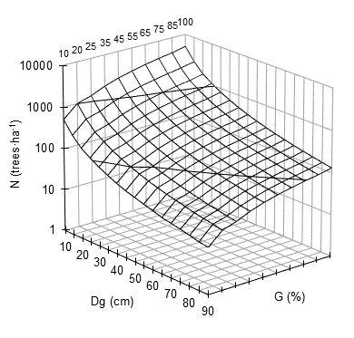
Figure 4 Maximum density lines for mixed-species stands of Durango, Mexico. Number of trees per hectare (N) against the mean square diameter (Dg) for the percentages of the basal area (G).
An average growth space diagram (AGSD) was created with the maximum density lines and growth zones corresponding to the DMD. The diagram represents the average growth space (S, m2) and the Dg (m) for the development of mixed stand trees (Pretzsch & Biber, 2005) in the growth zones (Figure 5). The combination of Dg and N corresponds to S in each line (Figure 3). In the line of maximum density (100 % of the SDI), for Dg = 20 cm and N = 1 603 trees·ha-1 there are S = 6.24 m2 and D = 2.49 m; in the line of imminent mortality (70 % of the SDI), for Dg = 20 cm and N = 1 042 trees·ha-1 there are S = 9.60 m2 and D = 3.098 m.
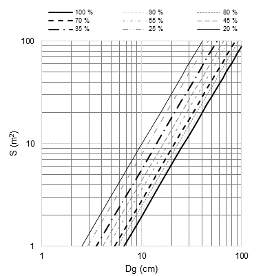
Figure 5 Average growth space diagram (S) against the mean square diameter (Dg) for mixed-species forests of Durango, Mexico.
The estimated value of the slope parameter (-1.86), obtained by OLS (Table 2), was more pronounced than the theoretical value of Reineke (-1.605), which is outside the 95 % confidence interval generated by OLS. This reinforces the argument that, for this case, the value of the slope is specific and varies with the species (Burkhart, 2013; Reineke, 1933), the characteristics of each region (Comeau et al., 2010) and the habits of growth of mixed-species stands. In addition, the OLS intercept confidence interval considers the value of the estimates obtained with SFR, and the value of the slope of SFR with N-T is statistically different from that of OLS adjusted at a confidence level of 95 %. The N-T approach, in the 95% confidence interval (-1.541 to 1.778), contains the theoretical value of -1.605 found by Reineke (1933). On the other hand, the line of maximum density is objectively adjusted (Bi et al., 2000) and the value of the slope is less pronounced than with OLS, due to the mixture of species and the adjustment procedure used (Sterba & Monserud, 1993).
In addition to the above, SFR provides a direct and efficient estimate of the upper limit of self-thinning (Santiago-García et al., 2013). Therefore, the adjustment with OLS is sensitive to the selection of data and can generate maximum density lines with inappropriate slopes (Reyes-Hernandez et al., 2013), because there is an intrinsic problem of subjectivity in the data selection of maximum density (Chen, Kang, Bai, Fang, & Wang, 2008). In contrast, SFR with N-T has the ability to fit the maximum density line at the upper limit of the dataset (Zhang et al., 2005), which implies that the line generated for mixed-species stands studied is consistent both statistically as biologically.
The maximum density line, obtained for the stands mixed with the SFR method and N-T approach, is above the upper limit of the density-size ratio from the dataset used. This result contrasts with that indicated by Zhang et al. (2005) in the sense that SFR adjusts the maximum density line below the upper limit of the experimental data; however, it coincides with that found by Santiago-García et al. (2013), who used the N-T procedure for P. patula in Hidalgo, Mexico. The graph behavior in log-linear scale (log-log) suggests the possibility of using a segmented model to characterize the dynamics of stands and episodes of mortality, as suggested by Cao and Dean (2008), who used a three-segment model for Pinus taeda L. and P. elliottii. The first segment characterizes the condition of the forest before mortality and the other two characterize mortality rates.
The zones defined in the DMD are compatible with the production zones of the Langsaeter theory (Langsaeter, 1941). Although there are differences between pure and even-aged forests and mixed and uneven-aged forests, in this study, the increase in the basal area was used to define the line of imminent mortality or self-thinning to 70 % of SDImax. The growth areas were delimited by the SDI: 1) in zone I (SDImax ≤ 20 %), the growth per unit area was proportional to the density (before crown closure) and the average basal area was 12.98 m2·ha-1; 2) in zone II (20 % < SDImax ≤ 35 %), the growth per unit area was proportional to the density, but the individual growth starts the decline, in this case, the average basal area was 27.21 m2·ha-1; 3) in zone III (35 % < SDImax ≤ 70 %), the growth per unit area is not proportional to the density, only the distribution, with an average basal area of 45.45 m2·ha-1 and 4) in the zone IV (70 % < SDImax ≤ 100 %), the growth per unit area is invariant of density; however, when it increases, net production decreases (Gilmore et al., 2005; Newton, 1997). For the generated DMD, the average basal area for the SDImax line was 64.93 m2·ha-1.
The prescription of thinning was programmed in the constant growth zone, in which the constant optimum density is given before crown closure (before self-thinning occurs) and can be assumed to maximize timber production and other forestry management objectives (Zeide, 2004). The lines of the DMD (Figure 3) have been defined for self-thinning between 55 and 66 % of the SDImax, the line of constant growth zone between 30 and 35 %, and the line of free growth between 13 and 20 % of the SDImax. These criteria have been used in studies for P. menziessii (Drew & Flewelling, 1979), Alnus rubra Bong (Hibbs, 1987), Abies balsamea (L.) Mill. , (McCarthy & Weetman, 2007), Pinus densiflora Siebold & Zucc., even aged stands of coniferous mixture (Newton, 1997) and P. patula (Santiago-García et al., 2013).
The optimal average growth space, in which the maximum potential of a site is used, is defined in the constant growth zone (35 to 70 % of the SDI), even though the density is affected by the variables used to measure the density (basal area, volume, mean square diameter or relative density) and the interpretations of such measures (Zeide, 2004). The properties in relation to these density approaches in a stand are associated with the ecological processes of growth and populations (Long & Vacchiano, 2013).
Conclusions
The maximum density line for mixed-species forests of Durango, Mexico, was created with a stochastic frontier regression approach, as a normal-truncated model. The density management diagram can be applied to prescribe thinning, regarding the development of mixed forest species in constant growth zone (zone III of the Langsaeter theory). In this zone, the optimal utilization of the site resources is guaranteed, and the thinning programs can be applied between 22.71 m2·ha-1 and 45.45 m2·ha-1 of average basal area, delimited by 35 to 70 % of the maximum stand density index (SDImax). This includes many combinations of trees per hectare and mean square diameter for the objectives of forest management and reconversion of species, as well as for the ecological and conservation of species diversity in mixed-species forests, which can be regulated during forest rotation. The implementation of the methodology to dispersal the general SDI of the species present in a stand, suggests that thinning can be programmed according to the global SDI. They can also be programmed per species to regulate their composition, through silvicultural treatments and the average growth space for mixed-species forests studied with timber production objectives.

