


 nueva página del texto (beta)
 Inglés (pdf)
 Artículo en XML
 Referencias del artículo
 Enviar artículo por email
 Citado por SciELO
  Similares en
SciELO
Similares en
SciELO 
 Permalink
Introduction
The Little pocket mouse, Perognathus longimembris Coues, occupies desertscrub habitats throughout the Great Basin, Mojave, Colorado, and western parts of the Sonoran deserts in western North America (Hall 1981). It also has a very limited occurrence in the California Floristic Province (CFP) along the Pacific coast in California (Cooper 1869). Infraspecific taxonomy has not been reviewed across the entire range since Osgood (1900); the only treatments subsequent to the last subspecies description (Hall 1941) are those for taxa occurring within Nevada (Hall 1946), Utah (Durrant 1952), and Arizona (Hoffmeister 1986). Of the 22 nominal taxa assigned to the species, recent taxonomic synopses have recognized either 15 (Patton 2005) or 16 (Williams et al. 1993; Hafner 2016) as valid, treating the remainder as synonyms. A thorough review of the species using modern morphological and molecular approaches is long overdue and also the subject of a larger review of the complex by one of us (JLP and collaborators).
Herein we examine the morphological disparity of Little pocket mice in one relatively small area of the species’ range, that across southern California and adjacent northern Baja California. In part, our treatment serves as a companion to available mitochondrial DNA views of population diversity across this same region (Swei et al. 2003). It also, hopefully, will serve as a taxonomic guidepost for population-level genomic studies now initiated by researchers at the San Diego Zoo Wildlife Alliance (Wilder et al. 2022) and the University of California Museum of Vertebrate Zoology, through the California Conservation Genomics Project (https://www.ccgproject.org/) and a refocus on taxa and areas of conservation concern for coordinated management decisions at the local, state, and federal levels.
Our area of interest includes six currently recognized subspecies: aestivus Huey, bangsi Mearns, bombycinus Osgood, brevinasus Osgood, internationalis Huey, and pacificus Mearns. This number represents 37.5 to 40 % of the valid infraspecific taxonomic diversity within P. longimembris but represents only about 10 % of the total species’ range (approximately 22,000 mi2 compared to 213,000 mi2). Despite the small encompassing area, high taxonomic diversity across this region is perhaps not surprising, as was found in a larger analysis of mammal “evolutionary hotspots” in California (Davis et al. 2008). Both ecological and topographic diversity are extreme, with five (of the 17) California ecoregions and four (of 11) geomorphic provinces included all or in part. The area also includes the only U.S. federally endangered pocket mouse (the Pacific pocket mouse, P. l. pacificus Mearns), now limited to only two small areas along the central coast in Orange and San Diego counties, and three of five other subspecies listed by the California Department of Fish and Wildlife as State Species of Special Concern, with a rank of S1 (Critically Imperiled) or S2 (Imperiled; CNDDB 2022).
Two of our six target taxa (pacificus Mearns and bombycinus Osgood) were originally described as distinct species and two were arranged under different specific epithets (arenicola Stephens and brevinasus Osgood allocated, as subspecies, to P. panamintinus Merriam); Williams et al. (1993) included all within their concept of P. longimembris. These authors also placed arenicola Stephens (following Grinnell 1913, 1933 and Huey 1928) and cantwelli von Bloeker (following Huey 1939 and Hall 1981) as junior synonyms of bangsi Mearns and pacificus Mearns, respectively. Of the six taxa Williams et al. (1993) treated as valid (pacificus Mearns, bangsi Mearns, brevinasus Osgood, bombycinus Osgood, aestivus Huey, and internationalis Huey), these authors regarded only internationalis as of equivocal validity. While California samples along the lower Colorado River are currently assigned to bombycinus Osgood (see Grinnell 1913, 1914, 1933; Hall 1981; and Williams et al. 1993), the type locality of this taxon is Yuma, Yuma County, Arizona, on the opposite bank. This river forms the dividing line between multiple subspecies and sister species of heteromyid and other rodents (e. g., Grinnell 1914; Hoffmeister and Lee 1967; Riddle et al. 2000).
Diversity among population samples of P. longimembris across the area has been examined, at least limitedly, by morphological and molecular characters. Over 80 years ago, Huey (1939), for example, compared adult specimens of all forms named above and provided tables of mensural character data, but his analyses were limited by small sample sizes, geographic coverage, and analytical scope. He noted (p. 49), however, while “an ultimate revision of the group” was required that “such a work is, owing to the considerable amount of material yet to be gathered, still in the distant future.” At the molecular level, Swei et al. (2003) showed that mitochondrial DNA diversity, while extensive within local populations, failed to recover any phylogeographic lineage structure among geographic samples assigned to pacificus Mearns, bangsi Mearns, brevinasus Osgood, and internationalis Huey. Species-wide mitochrondrial data now available (JLP, unpublished data) place the California populations allocated to bombycinus Osgood within the same mitochondrial group as those reported by Swei et al. (2003) yet indicate that this group of subspecies differs from topotypic and other samples of bombycinus across the lower Colorado River in Arizona. Unfortunately, no molecular data are yet available for aestivus Huey.
Huey’s “distant future” is today. The population-level genomic studies mentioned above will undoubtedly inform important issues of demographic history while identifying areas of isolation and/or genetic connectedness among extant populations. Eventually, these studies may also identify the underlying genetic basis for key morphological characters we describe below and provide a window into the role that selection has played in generating that diversity. We include analyses that center on colorimetric as well as standard mensural data of the skin and skull, to allow comparison to the limited published studies, and expand cranial analyses by using two-dimensional geometric morphometric approaches to delineate explicit shape differences. Our goal is to describe disparity among available population samples for each of the six taxa in our study area, to assess if the current taxonomy actually reflects geographically defined patterns of character variation, and to inform conservation understanding and management decisions if not.
Materials and methods
We examined a total of 721 museum specimens, of which we digitized 672 intact, adult skulls from 123 separate localities. These we grouped into 20 geographic samples (map, Figure 1; Appendix 1 provides provenance and catalog numbers) based on preliminary analyses that assigned nearby small samples into larger non-significant subsets as determined by oneway ANOVA and Tukey-Kramer post hoc tests. Seven of these samples comprise only the holotype (pacificusMearns, 1898 [USNM 61022], bangsi Mearns, 1898 [MCZ 5304; incorrectly listed as AMNH 5304 in Williams et al. 1993], arenicolaStephens, 1900 [USNM 99828], brevinasusOsgood, 1900 [USNM 186515], aestivusHuey, 1928 [SDNHM 6110], cantwelli von Bloeker, 1932 [MVZ 74680], and internationalis Huey, 1939 [SDNHM 11971]) and topotypes of each of the nominal taxa that have been described from our study area. We initially allocated samples to recognized subspecies following range limits given by Grinnell and Swarth (1913) and Grinnell (1933) rather than by Williams et al. (1993), who assigned specimens from San Gorgonio Pass (Banning east to Cabazon) to P. l. brevinasus not P. l. bangsi. We treated specimens from localities not included within each sample (black circles in Figure 1) as unknown.

Figure 1 Individual localities allocated to 20 regional samples of Perognathus longimembris across southern California and northern Baja California, color coded by subspecies allocation, and population within subspecies by symbol shape. Small black circles are localities with few, mostly singleton, specimens treated as unknown in canonical variate analyses. Arrows and asterisks identify the type locality of each of the seven named taxa allocated to P. longimembris in this area (listed by date and page priority: a = pacificus Mearns, b = bangsi Mearns, c = arenicola Stephens, d = brevinasus Osgood, e = aestivus Huey, f = cantwelli von Bloeker, g = internationalis Huey). Inset drawing of a Pacific pocket mouse by Tristan Edgarian.
Age criteria. We categorized age classes by maxillary tooth wear similar to the scheme employed by Hoffmeister (1986: Figure 5.131) for Arizona samples of P. longimembris, respectively: age class 0 - deciduous premolar 4 still in place or, if gone, permanent PM4 has not reached the molar occlusal plane; age class 1 - PM4 has reached occlusal plane of molar series but all cusps lack evidence of wear; age class 2 - cusps of PM4 and M1-M3 exhibit wear but remain separate or, if partially coalesced, have not unified into complete transverse lophs; age class 3 - cusps of posteroloph of PM4 and anterior and posterior lophs of M1 and M2 have coalesced into separate lophs that remain unconnected on their lingual boundary; age class 4 - anterior cusp of PM4 has coalesced with the posteroloph, lophs of M1-M3 are connected at their lingual border; and age class 5 - the occlusal surface of all teeth are “dished”, with enamel present only around the tooth’s border (occlusal patterns for age classes 2-5 are illustrated in Figure 2c).
Age classes 0 and 1 are considered to be juvenile animals based on porous auditory bullae and unfused basi-cranial sutures; age class 0 individuals are uniformly still in juvenile pelage and, for those specimens for which necropsy data are available, had not attained sexual maturity (i.e., females with thin and translucent uteri and males with very small, non-vascularized testes). Age class 1 individuals varied from still in juvenile pelage, in molt, or already with adult pelage; available necropsy data indicate that none had reached reproductive maturity. All specimens in age classes 2 through 5 had adult pelage and, especially in spring months, nearly all specimens with necropsy data exhibited signs of present or recent reproductive activity (females with enlarged, swollen uteri, embryos present, or embryo scars visible; males with enlarged, scrotal, and vascularized testes, and enlarged vesicular glands).

Figure 2 (a) Dorsal view of a skull of Perognathus longimembris (MVZ 240590; from East Stone Cabin Valley, Nye Co., Nevada) illustrating the position of 28 dorsal landmarks (LM - red circles) and the 21 semilandmarks (SL - yellow circles) that define the outer margin of the epitympanic (9 SL, black arc) and mastoid (12 SL, black arc) portions of the auditory bulla; (b) ventral view of the same skull with the positions of the 25 ventral landmarks indicated; and (c) maxillary toothrow occlusal surface wear age classes.
Non-geographic variation. To examine sex and age effects, we performed generalized least squares analyses of the 32 linear distance measurements for adult specimens of two samples: pacificus-1 (type and topotypes of pacificus Mearns; n = 66) and pacificus-3 (type and topotypes of cantwelli von Bloeker; n = 78). Application of Bonferroni corrections for multiple comparisons yielded no detectable sexual dimorphism nor significant interaction terms in either sample; significant age effects were found for four variables (nasal length, zygomatic breadth, upper incisor breadth, and mesopterygoid width) only in the pacificus-1 sample (Appendix 2). As a result, we combined sexes and ages in all analyses.
Cranial morphological character sets. We photographed the dorsal and ventral aspects of each skull examined using a Nikon D3200 or Nikon D850 digital camera fitted with AF-S AV Micro Nikkor 105 mm lens. Establishing a common plane for all photographed skulls is essential, whether photographs are used to calculate traditional linear measurements or digitized landmarks for geometric morphometrics. To maintain planar uniformity across specimens, we used a bubble level placed on the camera viewfinder and the platform upon which the skull was placed. For the dorsal view, the ventral surfaces of the bullae and the incisor tips established a common 3-point plane. A common plane for the ventral surface was more difficult to establish, as skulls were too small to use a bubble level laid across the molar rows, for example, and the age-related flattening of the dorsal profile made positioning each skull in a consistent position difficult. We thus placed each skull on a bit of putty and positioned the toothrows to a horizontal plane by eye. Damaged skulls that precluded digitizing all landmarks or accurate measurements, such as those with chipped incisors or broken parts, were excluded.
We digitized 28 landmarks (LM) on the dorsal surface of the skull and 25 on the ventral surface (Figure 2a, b) using the on-line XYOM-CLIC module (http://xyom-clic.eu/; Dujardin and Dujardin 2019). Most landmarks were Type 1 in Bookstein’s (1991) terminology - those where the intersection of bony sutures is locally defined; others conform to Type 2 as per Bookstein - those defined, for example, by the tip of a structure (dorsal LM 9, L26) or bulge (LM 6). In addition, we placed 21 semilandmarks (SL) along the lateral border of the auditory capsule, nine SL with uniform spacing between LM 13 and 14 along the edge of the epitympanic portion and 12 between LM 14 and 15 on the edge of the mastoid portion. We then used MorphoJ, version 1.07a (Klingenberg 2011; available at https://morphometrics.uk/MorphoJ_page.html) to generate matrices of Procrustes coordinates, or residuals, that result from superimposition, and principal components of the set of Procrustes residuals (or relative warp scores). MorphoJ uses the latter in canonical variate comparisons of a priori defined samples and to compute matrices of Mahalanobis distances among them. We also used MorphoJ to construct wireframes (sets of lines linking landmarks in a predetermined configuration) and deformation grids to visualize shape changes among taxon samples.
We also took 20 linear measurements from the dorsal surface, including the area (mm2) of the bullar capsule, and 12 measurements from the ventral surface from each skull photograph using ImageJ, version 1.46r (Abramoff et al. 2004; Schneider et al. 2012; available at http://imagej.nig.gov/if/download.html). ImageJ measurements were given to three decimals; these we rounded to two places, which is consistent with repeated measures of the same variable. Dorsal variables included: occipital-nasal length (1-ONL - midline distance from distal tip of ex-supraoccipital to anterior tip of nasal bones); nasal length (2-NL - midline length of nasal bones); frontal length (3-FL - midline length of frontal bones); parietal length (4-PL - midline length of parietal bones); interparietal length (5-IPL - midline length of interparietal bone); premaxilla tip length (6-premax-ExtL - midline measurement from the distal nasal bones to a line tangential to the two distal premaxillary extensions); rostral width (7-RW - width across the anterior rostrum at the nasal-premaxillary boundary); maxillary width (8-MW - width across the posterior rostrum at the maxillary-premaxillary boundary); premaxillary extension width (9-premax-tipW - width across the most distal portion of the premaxillary distal extensions); interorbital constriction (10-IOC - least width across the interorbital region); zygomatic breadth (11-ZB - maximum width across the zygomatic arches); anterior parietal width (12-antParietalW - maximum width of the parietal bones at their suture junction with the frontal and squamosal elements); anterior interparietal width (13-IPW-ant - maximum width taken at the suture junction with the parietal and ex-supraoccipital); posterior interparietal width (14-IPW-post - maximum width taken across the posterior corners of the interparietal); ex-supraoccipital width (15-exOccW - width across the exposed ex-supraoccipital elements); bullar width (16-bullarW - maximum width across the two bullae); bulla length (17-bullaL - maximum length from the anterior portion of the epitympanic and posterior portion of the mastoid portions); bulla width (18-bullaW - perpendicular width across the left bulla from the epitympanic-mastoid junction to the inner border with the ex-supraoccipital and parietal); bulla perimeter (19-bulla perimeter - the distance of a line circumscribing the left bulla); bulla area (20-bulla area - calculated for the area circumscribed by bulla perimeter, in mm2). Ventral variables included: anterior nasal extensions (21-anterior border of the upper incisors to the tip of the nasal bones); palatal length (22-posterior border of upper incisors to anterior end of mesopterygoid fossa); mesopterygoid length (23-anterior end of fossa to a line tangential to the posterior end of the hamular processes); foramen magnum length (24-midline measurement); maxillary toothrow length (25-alveolar length from upper premolar to third molar), incisor breadth (26-alveolar distance from the lateral margins of the incisors); palatal breadth (27-width across outside of maxilla between first and second molars); squamosal width (28-distance between the squamosal extensions); distal width of mesopterygoid (29-across the end of the hamular processes); stylomastoid foramina width (30-across the two stylomastoid foramina), occipital condyle width (31-across the distal ends of each condyle); ex-supraoccipital width (32-distance between the lateral projections of left and right ex-supraoccipital bones). External measurements of total length (TOL), tail length (TAL), hindfoot length, including claw (HF), and ear length, from notch (E) were taken from specimen labels; we calculated head-and-body length (HBL) by subtracting TAL from TOL.
We obtained dorsal and ventral landmark datasets for all digitized specimens of each taxon, although the final number in each differs slightly after removal of outliers. Sample sizes for ventral measurements were often smaller than those from the dorsum due to damaged structures (e. g., the hamular processes). In general, we employed linear variables primarily for comparisons to previously published studies that reported differences in cranial dimensions or to test character differences identified in diagnoses of taxa when initially described or subsequently compared.
Dorsal color measurement. Of the 721 specimens examined, 565 had preserved skins. These we photographed to obtain measures of the three Commission internationale de l'éclairage (CIE) color variables L* (lightness, measured on a scale from 0 [= black] to 100 [= diffuse white]), a* (the position on the color spectrum between red/magenta and green [negative values indicate green while positive values indicate magenta]), and b* (the position on the color spectrum between yellow and blue [negative values indicate blue and positive values indicate yellow]). To obtain these values, we first took photographs of the dorsal aspect of each skin at a distance of 25 cm using a Nikon DX SWM micro 1:1 lens and under standard lighting conditions at 4600oK; each photograph was then manipulated to yield an approximate uniform white background with L* = 90, a* = 0, and b* = 1. We then recorded, and averaged, color values at three points along the mid-dorsum from each specimen using the Lab Color Mode in Adobe PhotoShop CC™ (Adobe Systems Inc., San Jose, California). Since pelage color at any spot on the dorsum is variable due to a mixture of dark brown or black intertwined with yellow, individual measurements were an average of a 5 x 5 pixel area.
We converted values of a* and b* to C* (chroma, or relative saturation, which is measured on a scale from 0 to 100), as the square root of a*2 + b*2, and ho (hue, or angle of the hue in the CIELab color wheel), measured as the arctangent of (b*/a*). A red hue is at 0o, yellow at 90o, green at 180o, and blue at 270o, with orange, yellow-green, cyan, and magenta at 45o, 135o, 225o, and 315o, respectively).
Statistical procedures. We performed all multivariate analyses of landmark-semilandmark coordinates in MorphoJ but used JMP Pro16™ (SAS Institute Inc., Cary, North Carolina) for univariate character or multivariate specimen score comparisons among samples for morphometric and colorimetric data. We used oneway ANOVAs followed by Tukey-Kramer pairwise post hoc tests (with Bonferroni corrected P-values for multiple comparisons) in all comparisons of samples to delimit non-significant sample subsets. We also used the hierarchical clustering routine in JMP Pro16, with the Ward algorithm, to generate dendrograms from matrices of sample Mahalanobis distances and the canonical variates routine to obtain posterior probabilities for assignment for unknown specimens, those not allocated a priori to one of the 20 samples. The latter provided an unbiased assessment of each specimen phenetic relationship to a priori samples based on posterior probabilities of assignment. As multivariate ordinations of dorsal and ventral landmark datasets yielded similar patterns of sample dispersion in multivariate space, we present only those derived from the dorsal landmarks and semilandmarks. We performed all MorphoJ canonical analyses with permutation tests for pairwise distances with 10,000 iterations. The LSID for this publication is: urn:lsid:zoobank.org:pub:83CCE2F4-CE8C-4DB7-8116-50C83DA819F2.
Results
We begin by using the 32 linear variable dataset to examine character differences among the seven samples, which include the respective holotype and set of topotypes, or near-topotypes, of each nominal taxon in our study area. Here we wish only to evaluate the univariate characters used in the original descriptions or subsequent reviews upon which the current taxonomy has been based. We then examine disparity among all 20 samples mapped in Figure 1 and follow with analyses focused on more limited geographic areas where multivariate patterns of sharp transition are indicated in the global analysis. For these we employ only the dorsal landmark data since, as noted above, both dorsal and ventral landmark data illustrated the same ordination of samples. As we are interested in the phenetic relationships among samples, we only present results from canonical variates analyses.
Cranial characteristics of type and topotypic series. There are seven nominal taxa whose type localities are within the geographic area of our study (aestivus Huey, arenicola Stephens, bangsi Mearns, brevinasus Osgood, cantwelli von Bloeker, internationalis Huey, and pacificus Mearns), each within a separate sample (aestivus, bangsi-7, bangsi 2, brevinasus-1, pacificus-3, internationalis-1, and pacificus-1, respectively) that also contain the type series (if identified in the original description) and subsequently collected topotypes.
Earlier comparisons among these taxa centered on body and cranial size as well as the degree of mastoid bulla expansion with concomitant changes in lateral width of the interparietal and ex-supraoccipital bones. A few other cranial elements are mentioned in some accounts (for example, length and breadth of the nasals, or rostrum, and interorbital region), but these are limited to specific pairs of taxa and have not been reviewed across them all. In these limited comparisons, however, the series representing pacificus Mearns are uniformly stated to be exceedingly small in body and skull, darker in dorsal color, and with much smaller mastoid bullae, much wider interparietals, shorter rostra or nasals, and wider interorbital regions. In contrast, the series representing aestivus Huey is notable for being larger in body and cranial size, with much larger and inflated mastoid bullae that give a greater width to the posterior skull while compressing the interparietal into an almost equal-sided pentagon (e. g., Huey 1928). The other taxa fall varyingly with intermediate character states between the extremes represented by pacificus and aestivus.
Huey (1939:49) noted “structurally, there is found to be an entirely different trend of development” among the taxa he examined. Specifically, in contrasting samples from the coast and interior valleys through this region, he wrote “forms living nearest the ocean, such as pacificus near the shores of the Pacific and bombycinus … near the shores of the Gulf of California, have the smallest skulls. In fact, the mice themselves are the smallest members of the species. Those occupying the mountain areas are larger and show generally increasing size from north to south. The maximum size of the cranium is found in the specimens of aestivus, which occupies the western slopes of the Sierra Juarez and eastern end of El Valle de la Trinidad… Similarly, in the case of altitude, it is found that the greater the elevation, the greater the development of the bullae.”
These general observations are upheld in our comparisons among the type-topotypic series, as evidenced by the minimally non-significant sample subsets for external and selected cranial variables, along with character means, standard errors, and sample sizes provided in Appendix 3. In external characters, Mearn’s pacificus is the smallest in total length (mean = 119.64 mm), but Huey’s aestivus is largest only in hind foot length (mean 18.83 mm). There is, however, less uniformity among those cranial characters identified by describers and reviewers in the separation of these taxa. Both pacificus and cantwelli do have the smallest skulls (mean ONL = 19.83 and 19.76 mm, respectively; not significantly different from one another) with especially small bullae, but significantly smaller from one another (mean bulla perimeter = 17.32 and 16.61 mm); the interparietal of pacificus is especially wide (mean IPW-ant = 3.85 mm) but that of cantwelli is not (mean 3.55 mm). Conversely, aestivus does possess the largest skull (mean ONL = 21.57 mm) and largest bullae (mean bulla perimeter = 21.44 mm), significantly so, but shares long nasals with bangsi and internationalis (mean NL = 7.70 mm versus 7.67 and 7.57) and the narrowest interparietal with arenicola (both with mean IPW-ant = 3.10).
Global cranial disparity among all samples. We illustrate differences in dorsal cranial shape in Figure 3a, a biplot of canonical variate scores for the first two CVA axes. Below and to the left of these axes we present deformation grids, with vectors indicating compression or expansion of specific areas of the skull, and wireframe diagrams that compare the resulting shape differences between the most disparate samples aligned on each axis. In Figure 3b, we show the dendrogram of Mahalanobis distances among samples to illustrate hierarchical relationships among them.
The first two CV axes combine to explain 54.8 % of the total pool of variation; each additional axis explains < 8 %. Samples (Figure 3a) are ordered diagonally into three general groups that align separately on the two axes: (1) all Colorado Desert floor samples of bangsi and bombycinus plus aestivus; (2), interior basin samples of brevinasus and internationalis along with bangsi samples from San Gorgornio Pass; and (3) coastal samples of pacificus. The degree of overlap among samples differs but is notably divergent for the southern (pacificus-1) versus central and northern samples (pacificus-2 and -3) of pacificus. Both deformation grid and wireframe diagram for CV1 emphasize the correlated expansion of the bulla and compression of the posteromedial portion of the braincase, with the pacificus samples sharing a small bulla and wide interparietal and ex-supraoccipital relative to desert samples of bangsi, bombycinus, and aestivus. In contrast, CV2 emphasizes shape differences in the rostrum, notably contrasting the elongated nasals and narrowed distal premaxillary tips of bangsi samples with short nasals and wider premaxillary tips of pacificus. The dendrogram separates samples into the desert samples of bangsi (bangsi-1, -6, -7, and -8) and bombycinus plus aestivus versus all others. The latter is further subdivided, notably with all three pacificus samples grouped together, all northern bangsi samples (bangsi-2, -3, -4, and -5) grouped, and those allocated to brevinasus and internationalis split. Centroid size orders samples from largest (aestivus) to smallest (all three pacificus and the two bombycinus samples). Among-sample significant differences are present, but overall samples are ordered from large to small with overlapping non-significant subsets.
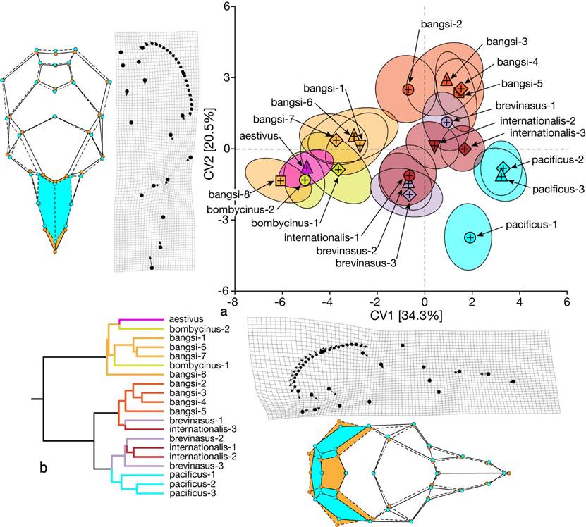
Figure 3 (a) Biplot of canonical variate scores (CV) for the first two axes of dorsal skull landmarks for all 20 samples of Perognathus. longimembris from southern California and northern Baja California; data are presented as sample means (+) and ellipses that encompass 50 % of specimen scores. Below and to the left are deformation grids for the left side of the skull, which contains the semilandmarks conforming to the bulla perimeter, and wireframe diagrams of the entire skull, excluding the semilandmarks, with colored highlights of cranial areas of major change that compare samples from the extremes on each axis. (b) Dendrogram of Mahalanobis distances depicting hierarchical similarities among all samples. Symbols and colors are those in the map, Figure 1.
The combination of CV1 scores and centroid size (lognCS; Figure 4) cleanly separates those samples from the desert floor from those of the coast and interior valleys in y-intercept and slope (z = 5.31, P < 0.001 and 2.19, P < 0.01). The single exception is Huey’s aestivus, which, while occupying the western base of the Sierra Juarez in northern Baja California, shares characteristics of the desert samples. This relationship is contrary to that posited by Huey (1939:49) in his contrast of coastal and interior populations and taxa.
Cranial disparity across transition areas. Three features of the landmark analytical results deserve comment. First, morphological disparity across the entire sample area reveals two primary groupings of samples: those of the coast, interior valleys, and San Gorgonio Pass and those of the lowland deserts to the east, including the sample from northern Baja California (Figures 3 and 4). Second, there are several geographic areas of sharp transition, both within and between these two geographically structured groups, but also among samples allocated to the same subspecies. And third, samples bordering these sharp transition areas often contain individual specimens that span the mean morphological gap, suggesting phenotypic intermediacy derived from gene flow. Here we examine more closely these transitional areas through CVA. These analyses also permit us to allocate those unknown specimens listed in Appendix 1 by their posterior probabilities to one of the included a priori samples. We organize these analyses by focusing first on transitional areas between the two primary sets of samples identified in figures 3 and 4, specifically (1) internationalis versus adjacent bangsi samples and (2) bangsi versus desert samples. We then consider transitional areas within each of the two global subsets, between (3) coastal pacificus versus interior basin brevinasus + internationalis, (4) brevinasus versus bangsi samples across San Gorgonia Pass, and (5) northern Baja California aestivus versus desert samples of bangsi + bombycinus. The degree of differentiation across each of these transitions will inform a concluding set of systematic decisions regarding units that warrant taxonomic recognition as well as the geographic range of each. In turn, our suggested taxonomic units will inform conservation status of some, notably pacificus and bangsi.

Figure 4 Plot of CV1 scores on log centroid size (lognCS) for the 20 samples of Perognathus longimembris depicted in Figure 3. Regression lines, with 95% confidence limits, and equations are provided. Symbols and colors are those in the map, Figure 1.
1-Southern interior valleys and adjacent desert floor. This area encompasses the phenotypic disparity among the three, southern-most bangsi (-6, -7, and -8) and the three internationalis samples that are geographically adjacent on the desert floor and interior valleys, respectively (Figure 1). We used the same approach as above, deriving CV scores from CVA in MorphoJ for those specific samples. The combination of CV1 and CV2 scores separates the two taxa on the first axis and orders within-taxon samples geographically (bangsi samples from north to south, internationalis samples from south to north) on the second (Figure 5a); these two axes combine to explain 70 % of the variation. Samples of bangsi have a proportionally longer but posteriorly narrowed rostrum, narrowed frontal and parietal elements, and larger bullae coupled with narrowed interparietal and ex-supraoccipital bones in comparison to those of internationalis (see Figure 5a, wireframe diagram). Regression relationships of centroid size (lognCS) on CV1 scores separates the pooled taxon samples (Figure 5b), with significant differences in mean values, y-intercepts, and slopes. The internationalis samples are significantly larger in centroid size (pooled internationalis lognCS mean = 3.609, pooled bangsi = 3.573; oneway ANOVA P < 0.001); the two separate along CV1 (mean eigenvector 1.761 versus -1.952, respectively; P < 0.001; y-intercept (34.549 versus -16.504; P < 0.01); and slope -9.084 versus 4.073; P < 0.01).
The two northern-most bangsi samples, however, do broadly overlap with their geographic internationalis counterparts, with specimens from each spread across their respective 75 % inclusion ellipses (Figure 5a). This suggests either past and/or present gene exchange between Mason Valley (internationalis-2) and San Felipe Valley (internationalis-3) with San Felipe Narrows (bangsi-7) and Borrego Valley (bangsi-6), perhaps along San Felipe Creek, which connects these areas today. In contrast, there is no overlap of 75 % inclusion ellipses nor are specimens of either misplaced between the southern-most internationalis sample (internationalis-1), which contains the holotype and type series from the vicinity of Jacumba, and the few available specimens from localities in the Yuha Desert region that span the international border (bangsi-8). The samples of bangsi and internationalis thus become progressively more differentiated from north to south along their respective ranges.

Figure 5 (a) Biplot of canonical variate scores of the first two axes of dorsal cranial landmarks for southern samples of bangsi and geographically adjacent samples of internationalis; data are presented as sample means (+) and ellipses that encompass 75 % of specimen scores (open ellipses) and 95% confidence limits around the mean (colored ellipses). Below is the wireframe diagram depicting areas of dorsal cranial differentiation highlighted in color comparing bangsi (dashed lines, cranial elements in pale orange) with the combined internationalis samples (solid lines). (b) Linear regression, with 95% confidence limits, of CV1 scores on log centroid size (lognCS); large crosses indicate mean values. Symbols and colors are those in the map, Figure 1.
2-San Gorgonio Pass and Colorado Desert samples. Here we examine the relationships among samples of bangsi Mearns (bangsi-1 through -8) and bombycinus Osgood (bombycinus-1 and -2) from San Gorgonio Pass east through desertscrub vegetation on the floor of the Colorado Desert of southeastern California (Figure 1). As above, we conducted CVA and illustrate the biplot of CV1 and CV2 scores (which combine to explain 71.2 % of the total variation; note that CV1 alone explains 60.3 %) in Figure 6a. Desert floor samples of bangsi and bombycinus have much larger bullae that project distally from the occiput and, conversely, laterally compressed interparietal and ex-supraoccipital elements (Figure 6a, wireframe diagram). Regression relationships of centroid size (lognCS) on CV1 scores again separates the pooled taxon samples (Figure 6b), with significant differences in mean values, y-intercepts, and slopes. San Gorgonio Pass samples of bangsi are significantly larger in centroid size (pooled samples bangsi-2 through -5, lognCS mean = 3.597; pooled desert samples = 3.569; oneway ANOVA P < 0.001); the two separate along CV1 (mean eigenvector -2.074 versus 2.547, respectively; P < 0.001; y-intercept (-8.695 versus 38.390; P < 0.05); and slope 1.840 versus -10.040; P < 0.01).
The ordination of samples, however, is less discrete than in the previous transition zone analysis, with broader overlap of specimens among samples from the San Gorgonio Pass (bangsi-3 through -5) and the geographically adjacent type and topotype series from Palm Springs (bangsi-2). The bangsi samples on the desert floor to the immediate east (bangsi-1) and south (bangsi-6 and -7) along the desert side of the Peninsular Ranges overlap partially with the cluster of bangsi-2 through -5, with the two bombycinus from the western side of the lower Colorado River, and the bangsi-8 sample from the Yuha Desert region. There is broad overlap between desert floor bangsi (bangsi-1, -6, -7, and -8) and the two eastern bombycinus samples along the first CV axis. Despite the overlap of adjacent sample individual specimens, there remains clear separations between the northwestern bangsi samples (bangsi-2 through -5) and all samples from the floor of the Colorado Desert, with a relatively sharp transition in shape of the distal cranial elements of the bulla, interparietal, and ex-supraoccipital (Figure 6a, wireframe diagram).

Figure 6 (a) Biplot of canonical variate scores of the first two axes of dorsal cranial landmarks for San Gorgonio Pass and lowland desert samples of bangsi and the desert bombycinus; data are presented as sample means (+) and ellipses that encompass 75 % of specimen scores (open ellipses) and 95 % confidence limits around the mean (colored ellipses). Below is the wireframe diagram depicting areas of dorsal cranial differentiation highlighted in color comparing northwestern bangsi (samples bangsi-2, -3, -4, and 5; dark orange circles, dashed lines, and orange cranial elements) with the combined desert samples of bangsi and bombycinus (pale orange circles, solid lines). (b) Linear regression, with 95 % confidence limits, of CV1 scores on log centroid size (lognCS); large crosses indicate mean values. Symbols and colors are those in the map, Figure 1.
3-Coastal versus interior valley samples. This analysis includes the three coastal samples (pacificus-1, -2, and -3) and six from interior valleys (brevinasus-1, -2, -3 and internationalis-1, -2, and 3) that separate from all desert samples further to the east across southern California (see Figure 3 and Figure 4). We again used canonical analyses to compare the nine samples and then samples pooled by subspecies allocation (Figure 1). We included all unknown specimens (Appendix 1) to determine their respective assignments in the two analyses.
The first two CVA analyses separate the three coastal samples and those from the interior valleys; for simplicity, we present data for only the 9-group analysis (Figure 7a). The first two axes are nearly equivalent in the percentage of the variation explained (32.1 and 29.1 %, respectively, or 62.2 % combined). While the ordination of samples is similar to that depicted in Figure 3, and with the same cranial features emphasized in this separation (compare wireframe in Figure 7a with that in Figure 3a), the degree of disparity in dorsal shape attributes is much less. These differences, nonetheless, do emphasize the smaller auditory bullae with the laterally expanded interparietal and ex-supraoccipital region along with the short and distally broader rostral elements of the coastal samples, pacificus-1, -2, and -3. Note the distinction between the pacificus-1 (which contains the type of pacificus Mearns) and paired pacificus-2 and -3 samples (the latter which contains the type of cantwelli von Bloeker). The two samples of pacificus versus brevinasus + internationalis also differ in their relationship of centroid size (lognCS) and CV1 scores (Fig 7b; mean lognCS coastal = 3.786, interior = 3.838; mean CV1 coastal = 1.483, coastal = -1.620; ANOVA P < 0.001 in each comparison), similar to that of the global analysis (Figure 4). In contrast, pooled samples of brevinasus and internationalis share the same means, y-intercepts, and slopes (P > 0.05), with each of those measures, except regression slope, differing from those values for the pooled pacificus samples (P < 0.001 in each comparison).
Assignments of unknown specimens are unambiguous. The three specimens from San Fernando, Los Angeles County (Appendix 1), are assigned to pacificus, specifically sample pacificus-3, at posterior probabilities above 0.948 in the 9-sample and pooled-taxon analyses. In contrast, all specimens from Riverside (Eden Hot Springs, Hemet, Temecula, and Vallevista) and San Diego (McCain Valley and Warner Pass) counties are assigned to the combination of brevinasus and internationalis samples at posterior probabilities > 0.861. The placement of each is illustrated in Figure 7a, b (black circles are individuals from San Fernando assigned to pacificus-3; black squares are those from Riverside and San Diego counties).
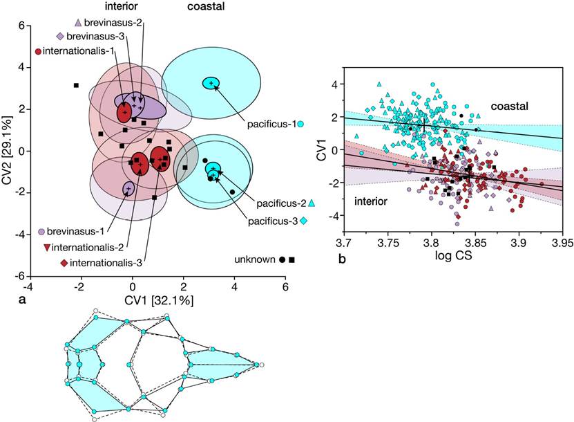
Figure 7 (a) Biplot of canonical variate scores of the first two axes of dorsal cranial landmarks for coastal pacificus samples and interior valley samples of brevinasus; data are presented as sample means (+) and ellipses that encompass 75 % of specimen scores (open ellipses) and 95 % confidence limits around the mean (colored ellipses). Below is the wireframe diagram depicting areas of dorsal cranial differentiation highlighted in color comparing pacificus (solid lines, elements in blue) with the combined brevinasus and internationalis samples (dashed lines). (b) Linear regression, with 95 % confidence limits, of CV1 scores on log centroid size (lognCS); large crosses indicate mean values. Symbols and colors are those in the map, Figure 1.
The separation of the three coastal samples into two quite distinct geographic groupings was unexpected. All are currently allocated to the endangered Pacific pocket mouse (P. l. pacificus) yet, importantly, all three currently known localities of this mouse are located within the pacificus-2 sample area (two on Camp Pendleton and Dana Point), which aligns with the northern part of this subspecies range (the pacificus-3 sample, which contains the holotype of cantwelli von Bloeker) rather than with the southern-most area (pacificus-1 sample) where Mearn’s holotype of pacificus was collected. We thus wished to ascertain to what degree, if any, the pacificus-2 sample might be divided into southern (pacificus-1 = pacificus) and northern (pacificus-3 = cantwelli) sets of individuals. We thus performed a CVA with these two sample sets as a priori groups and treated all specimens from the pacificus-2 sample as unknown. Only singleton specimens from either the pacificus (n = 63, Appendix 1) or cantwelli (n = 78) samples were misclassified. Among the 48 pacificus-2 specimens, 41 (85.4 %) were assigned to cantwelli at posterior probabilities > 0.70 (mean posterior probability assignment = 0.9796). Seven specimens were assigned to pacificus at posterior probabilities of 0.775 or higher (mean assignment = 0.9231). All assignments to pacificus came from the southern-most localities in the pacificus-2 sample (Oceanside [3 of 26 specimens], 4 mi N Oceanside [1], Santa Margarita River [1], and Santa Margarita Ranch [2]). The four specimens from the northern-most locality of Dana Point were each assigned to cantwelli at posterior probabilities > 0.996.
4-San Gorgonio Pass transect. Here we examine phenetic relationships among the type and topotypic specimens of brevinasus from the vicinity of San Bernardino (sample brevinasus-1) east across San Gorgonio Pass (the three samples of bangsi from Banning [bangsi-5], Cabazon [bangsi-4], and then Whitewater-Snow Creek [bangsi-3]) plus the type and topotypic specimens of bangsi from the vicinity of Palm Springs (bangsi-2). Given differences in subspecies allocation of this set of samples by Grinnell and Swarth (1913; see also Grinnell 1933) and Williams et al. (1993), we are specifically interested where phenotypic gaps might be found.
The first two CV axes combined explain 76.4% of the variation (Figure 8a) with the brevinasus sample separating from the four samples from San Gorgonio Pass along the first axis and the latter ordered from east (bangsi-2, top) to west (bangsi-5, bottom) on the second axis. Skulls of the different sample sets exhibit more subtle shape differences despite the separation of brevinasus from all four bangsi samples (Figure 8a, bottom wireframe diagram), with limited specimen overlap between brevinasus and its immediate bangsi neighbor from the vicinity of Banning (bangsi-5). Differences among the bangsi samples along CV2 separate bangsi-2 from the three samples located within San Gorgonio Pass, each geographically adjacent pair of samples with more substantial specimen overlap, mostly by changes in the posterior parts of the skull (bullae, interparietals, and ex-supraoccipitals; Figure 8a, wireframe diagram to the left), the same traits that continue the east to west trend illustrated in Figure 6a. The degree of the bangsi sample differences along CV2 is nearly as great as that between the two presumptive subspecies (CV1).
The relationship of centroid size (lognCS) to CV1 scores separates the sample of brevinasus from the pooled samples of San Gorgonio bangsi (Figure 8b). The bangsi samples are marginally larger in centroid size (pooled bangsi lognCS mean = 3.598, brevinasus = 3.590; one way ANOVA P = 0.03) and the two separate along CV1 (-0.991 versus 2.764, respectively; P < 0.001; y-intercept (-5.253 versus -27.453; P < 0.01) but not in slope 8.409 versus 1.184; P > 0.05).
As a final comment, the type-topotypic series of brevinasus (sample brevinasus-1) do not have the shorter nasal bones implied by their name. ANOVA comparisons of the nasal length of brevinasus-1 with each bangsi sample in this transect, as well as those of internationalis, are universally non-significant (pairwise P-values range from 0.546 to 1.000); in comparison to pacificus, brevinasus has longer nasals, actually and proportionally (P < 0.001 in each comparison).
5-Relationship of aestivus to desert bangsi and bombycinus. This final set of comparisons focuses on the desert samples of bangsi and bombycinus plus the northern Baja California aestivus, those samples that collectively contrast with coastal and interior ones in a dendrogram of among-sample Mahalanobis distances (Figure 3) and in relationships of their centroid sizes with CV1 scores (Figure 4). Huey (1928:87) diagnosed aestivus by its large and inflated mastoid bullae that gave it “a much greater width to the skull posteriorly and compressing the interparietal into an almost equal-sided pentagon.” While Huey was certainly correct, these same traits apply to desert bangsi samples (the eastern-most bangsi-1 and southern bangsi-6, -7, and 8) as well as the two bombycinus samples. The major difference, however, is that the skulls of aestivus are largest, bombycinus are smallest, and bangsi samples are intermediate in size (mean ? standard error for lognCS: aestivus = 3.623 ? 0.006, pooled desert bangsi = 3.579 ? 0.003, and pooled bombycinus = 3.529 ? 0.006). Furthermore, aestivus is broader across the mastoids (bullarW mean = 12.60 mm) than either bangsi (range 11.87 mm [bangsi-1] to 11.58 mm [bangsi-6]) or bombycinus samples (11.48 mm and 11.33 mm, respectively).
The CVA comparing these seven samples provides limited resolution among them. It takes the first four axes to explain nearly 75 % of the total variation. The first three axes individually explain only 28.5, 18.8, and 15.0 %, respectively. In the biplots of CV1 and CV2 or CV1 and CV3 (Figure 9a, b), most samples align from left to right, along the first CV axis while CV2 and CV3 separate the aestivus and one bangsi (bangsi-8) samples, respectively. Other combinations of CV axes simply shuffle the positions of these two samples with respect to the core group illustrated in Figure 9 (data not shown). Overall, there is limited resolution on any pair of axes and no clear, well-supported separation among this set of samples.

Figure 8 (a) Biplot of canonical variate scores of the first two axes of dorsal cranial landmark for brevinasus and bangsi samples west to east across San Gorgonio Pass; data are presented as sample means (+) and ellipses that encompass 75 % of specimen scores (open ellipses) and 95 % confidence limits around the mean (colored ellipses). Below is the wireframe diagram depicting areas of dorsal cranial differentiation highlighted in color comparing brevinasus (brevinasus-1; purple circles, solid lines, and colored cranial elements) with samples of bangsi from the Palm Springs area (bangsi-2) west across those within San Gorgonio Pass (bangsi-3, -4, and -5; orange circles and dashed lines). To the left is the wireframe comparing the bangsi-2 (orange circles and solid lines) sample with the other three (orange squares, dashed lines, and colored cranial elements). (b) Regression plot of CV1 scores on log centroid size (lognCS). Regression lines, with 95% confidence limits, and equations are provided. Symbols and colors are those in the map, Figure 1.
Pelage color disparity. We provide means, standard errors, sample size, and non-significant sample subsets based on Tukey-Kramer pairwise comparisons in Appendix 4. All three color variables (lightness, chroma, and hue) vary significantly across the sampled populations (oneway ANOVAs, P < 0.001 for each). Lightness varies from quite dark (mean L* = 13.99 [pacificus-1]) to very pale (46.53 [bangsi-1]) and chroma is ordered in the same way, from lower (in the pacificus-1 sample, mean chroma = 9.442) to higher purity (in bangsi-1, 21.855). Hue varies only negligibly among samples (lowest for pacificus-1 [mean 1.083] and highest in bangsi-6 [1.378]), with all specimens within the red spectrum (sample descriptive statistics in Appendix 3). Overall, the pacificus samples differ significantly from interior and, especially, desert samples in all three attributes; visually these are easily distinguished by their very dark overall tones; interior samples are intermediate, and desert ones are distinctly lighter.
In PCA and CVA analyses, the first axis explains the vast majority of the total pool of variation (PC1 = 94.75 %; CV1 = 88.31 %), with lightness the only variable that loads significantly on each axis (PC1 eigenvalue = 0.9541 [versus -0.2996 and -0.0041] for chroma and hue, respectively; CV1 standardized scoring coefficient = 0.9867 [versus 0.0246 and 0.001]). These two multivariate methods display the same ordination of samples, whether these are determined a posteriori (PCA) or a priori (CVA); correlation of specimen PC1 and CV1 scores = 0.998, ANOVA P < 0.001. Unsurprisingly, specimen lightness also predicts their individual PC1 and CV1 scores with high efficiency with correlations of 0.997 and 0.999, respectively. One does not need multivariate statistics to see, by eye, differences in pelage lightness among these samples, which we depict as box plots in Figure 10. While some samples are hampered by low numbers of available skins (notably eastern and southern desert bangsi-1 and -8, and bombycinus-1 and -2), the pattern of increasing lightness from coast to desert is obvious. Coastal samples are uniformly darkest but still separate into two significant groups, southern pacificus-1 versus central and northern pacificus-2 and -3 (Figure 10, black bars, which depict non-significant subsets based on Tukey-Kramer HSD). The color separation of these samples mirrors that of their cranial shape (Figs. 3 and 7). Interior basin samples of brevinasus and internationalis, individually and as a group, are also dark, significantly lighter than coastal pacificus but statistically uniform; samples of bangsi from west to east across the San Gorgonio Pass form a cline between darker interior and the very light desert samples. Regression of specimen L* values for the San Gorgonio Pass localities against longitude is significant (R2 = 0.307, df1,143, F = 62.93, P < 0.001). This observation is consistent with Grinnell and Swarth’s (1913:360) statement that some specimens from Banning (sample bangsi-5; Figure 1) “show slightly the darkest coloration, perhaps indicating intergradation towards brevinasus” and, along with cranial uniformity (Figure 8), support these authors’ allocation of specimens from San Gorgonio Pass to bangsi rather than to brevinasus (contra Williams et al. 1993).

Figure 9 Biplots of canonical variate scores of dorsal cranial landmarks for lowland desert samples of bangsi and bombycinus plus the northern interior valley sample of aestivus; data are presented as sample means (+) and ellipses that encompass 75 % of specimen scores (open ellipses) and 95 % confidence limits around the mean (colored ellipses): A - CV1 and 2 plot; B - CV1 and 3 plot. Symbols and colors are those in the map, Figure 1.
Discussion
We organize this section around two important, and interrelated, components of systematic research. The first addresses broad patterns, and degrees, of cranial and color disparity across the sampled region based on the separate transitional area analyses. This is a necessary first-step before tackling the second component, that of the optimal taxonomy that expresses the disparity of the patterns observed. Following these two components, we then posit historical biogeographic factors that might underly the cranial and pelage color disparities we recovered. We then end with potential management considerations as a result of our suggested taxonomic changes, and with a lament that so much of the original ranges of several of the taxa we include have disappeared under concrete and buildings, or been impacted by recent fires, each of which have changed the landscapes and habitats available for pocket mice and many other organisms, some irreversibly. Nonetheless, we believe it important to describe original patterns and processes of organismal diversification even if these exercises are only depictions of the past, not the future.
Synthesis of morphological disparity among samples. Samples of Perognathus longimembris from southern California and northern Baja California are diverse in cranial shape and pelage color, but the patterns are somewhat complex yet still geographically ordered. Here we map (Figure 11a) the major axes of cranial shape differentiation that derive from the global analysis (Figs. 3 and 4) and those of the individual transition areas (Figs. 5 - 9). The major axis of differentiation (heavy solid line in Figure 11a) separates eastern (desert plus aestivus) samples from those of the coast and interior valleys. Bridges between these two groups are evident in samples bangsi-2 vis-à-vis adjacent samples bangsi-1 to the east, bangsi-3 to the west, and bangsi-6 to the south (Figure 6), and between bangsi-6 and internationalis-2 (Figure 5). Secondary axes of differentiation occur between samples of coastal pacificus relative to the interior brevinasus and internationalis (Figure 7), and brevinasus (from the San Bernardino Valley) and bangsi samples (from San Gorgonio Pass; Figure 8). Tertiary levels of divergence occur among the three pacificus samples, which separate pacificus-1 (the type and topotypic series) from pacificus-2 and -3 from the central and northern coast, respectively (Figure 7). The array of brevinasus and internationalis samples, while grouped together, do not exhibit an expected clinal phenetic pattern but rather present as coupled pairs (Figure 7). Eastern desert samples of bangsi and bombycinus, including aestivus, are collectively less cohesive but, at least with available samples, they are not subdivided (Figure 9).
Dorsal pelage color, dominated by lightness (L*), exhibits the same geographic pattern as cranial shape (compare Figure 10 with Figs. 4 - 9). We have cranial and color data for 358 specimens. For these, we used linear regression to examine the correspondence between individual specimen cranial shape and color CV1 scores (Figure 11b). The relationship between these independent traits is strong (R2 = 0.4473, df1-357, F = 288.13, P < 0.001); specimens from each sample group together and array along the regression line in the consistent coastal to interior to desert pattern.

Figure 10 Box plots of pelage lightness, with means and specimen values, for samples of Perognathus longimembris from southern California. Samples are arranged from left to right: coastal (pacificus), interior valleys (internationalis and brevinasus), San Gorgonio Pass (bangsi, samples 2 through 5), and desert (bangsi, samples 1, 6, 7, and -8, bombycinus, and including aestivus from interior valleys of northern Baja California). Separate heavy lines above samples groups are non-significant subsets (oneway ANOVA, Tukey-Kramer HSD P > 0.05). Symbols and colors are those in the map, Figure 1.
Taxonomic implications. As the existing subspecific taxonomy implies (Williams et al. 1993, Patton 2005, Hafner 2016), phenotypic diversity across the entire sample area is substantial. In our opinion, available data support the recognition of four to six infraspecific units, listed below, but also a reshuffling of the current assignments of several populations. Coastal pacificus possess the most distinctive skull, with its small overall size, very small bullae and concomitant wide interparietals and supraoccipitals, and short rostrum; its recognition should certainly be retained. A lingering question, however, is whether this taxon should be subdivided, with the name pacificus Mearns applied only to the area around its type locality in extreme southwestern San Diego County, and cantwelli von Bloeker resurrected to encompass the coastal samples in northwestern San Diego and southwestern Orange counties and those around its type locality of Hyperion (= El Segundo) in Los Angeles County. We believe subdivision is warranted as pacificus (sensu stricto) and cantwelli differ in multiple morphometric, shape, and color attributes, and at a degree consistent with differences among other subspecies recognized (see Figures. 3 and 7, Appendix 3 and 4).

Figure 11 (a) Isophenes of cranial differentiation among samples of Perognathus longimembris from southern California and northern Baja California derived from canonical variate analyses presented in Figures 3 through 9. Differentiation is hierarchical, with the heavy line separating regional samples, light solid lines separating units within the western region, and dashed lines separating or grouping samples within current subspecies, but names are provided for infraspecific units we recognize herein. Symbols and colors are those in the map, Figure 1. (b) Regression plot, with 95 % confidence limits around the slope, illustrating the correspondence of individual specimens, as assigned to samples, for dorsal pelage color and cranial shape. Symbols and colors are those in the map, Figure 1.
Lacking any clear distinction between the six interior samples into northern and southern units that would map to the current taxa brevinasus Osgood and internationalis Huey, respectively, as well as the broad overlap among them, we recommend placing both under the earlier described brevinasus Osgood. Such action is consistent with the suggestion of equivocal recognition of the two by Williams et al. (1993). We suggest that samples allocated to bangsi Mearns be restricted to those in San Gorgonio Pass and the Whitewater River outwash, which includes the type locality of Palm Springs. Even though the type and topotypic series share phenetic similarities with samples to the immediate east (Shavers Valley) and south (Borrego Valley), those relationships are more distant than between the Palm Springs and San Gorgonio Pass samples. Eastern and southern bangsi samples, which grade into those allocated to bombycinus Osgood in the low eastern desert along the western margin of the lower Colorado River, are best considered a single unit. Given that the type locality of Osgood’s bombycinus is from Yuma, on the Arizona (eastern) side of the lower Colorado River, samples of which are molecularly and phenotypically distinct (JLP, unpublished data), the southeastern California samples cannot be referred to bombycinus. Fortunately, the bangsi-7 sample includes the holotype of arenicola Stephens; this name is available for these desert populations. As noted by Stephens in his original description, arenicola differed from typical bangsi by more swollen mastoids that project further posteriorly from the occiput, key features that are demarcated in our analyses (e.g., see wireframe diagram in Figure 6a). Until molecular data are available, we would provisionally retain aestivus Huey despite its cranial phenotypic overlap with these desert samples. We note that these suggested rearrangements will impact current conservation strategies for several of these pocket mice. Taxonomy is meant to inform, not to be derivative of those needs. A shortened listing of the valid taxa in southern California and northern Baja California, with range limits, is the following:
Perognathus longimembris pacificusMearns, 1898
1898. Perognathus pacificus Mearns, Bull. Amer. Mus. Nat. Hist., 10:299, 31 August.
1932. Perognathus longimembris pacificus: von Bloeker, Proc. Biol. Soc. Washington, 45:127 (first use of current name combination).
Type locality. “Edge of the Pacific Ocean, at the last Mexican boundary monument (No. 258), [San Diego County, California].”
Range. Currently limited to the estuary of the Tijuana River in immediate vicinity of Boundary Monument 258 to 3.2 km north of the monument, San Diego Co., California; likely extends, or used to, even further north along the coast and possibly eastward up the Tijuana River drainage, including into extreme northwestern Baja California, Mexico. Includes localities in sample pacificus-1 (Appendix 1).
Remarks. To our knowledge, this taxon was last collected in the wild in July (von Bloeker 1931b) and October of 1931 (W. H. Burt, Dickey Collection, University of California, Los Angeles).
Perognathus longimembris bangsiMearns, 1898
1898. Perognathus longimembris bangsi Mearns, Bull. Amer. Mus. Nat. Hist., 10:300, 31 August.
1900. Perognathus panamintinus bangsi: Osgood, N. Amer. Fauna, 18:29.
Type locality. “Palm Springs, Colorado Desert [Riverside Co.], southern California.”
Range. Limited to San Gorgonio Pass (the vicinity of Banning east to Cabezon, Snow Creek, and Whitewater) and outwash of the Whitewater River to the vicinity of Palm Springs, Riverside Co., California. Includes localities of samples bangsi-2, bangsi-3, bangsi-4, and bangsi-5. Localities from San Gorgonio Pass were allocated to brevinasus Osgood by Williams et al. (1993) but to bangsi by Grinnell and Swarth (1913); some, but not all, specimens from Banning share the darker pelage characteristic of that subspecies but cranially pool with other bangsi samples from the Pass.
Perognathus longimembris arenicolaStephens, 1900
1900. Perognathus panamintinus arenicola Stephens, Proc. Biol. Soc. Washington, 13:153, 13 June.
1918. P[erognathus]. l[ongimembris]. arenicola: Osgood, Proc. Biol. Soc. Washington, 31:96 (first use of current name combination).
Type locality. “San Felipe Narrows, San Diego Co., California.”
Range. Colorado Desert of eastern California and northeastern Baja California, from Shavers Valley east to Blythe (Riverside County) and Borrego Valley south to the Yuha Basin and east to Pilot Knob (Imperial County); range in Baja California unclear but probably extends south along the coast of the Sea of Cortez at least to San Felipe. Includes localities in samples bangsi-1, bangsi-6, bangsi-7, bangsi-8, bombycinus-1, and bombycinus-2.
Remarks. Treated as a synonym of P. l. bangsi by Grinnell (1913, 1933), Hall (1981), and Williams et al. (1993). May include aestivus Huey, pending molecular data if and when available. Grinnell (1914) assigned specimens from the vicinity of Pilot Knob to P. l. bombycinus, the type locality of which is in Arizona (see above).
Perognathus longimembris brevinasusOsgood, 1900
1900. Perognathus panamintinus brevinasus Osgood, N. Amer. Fauna, 18:30, September.
1928. Perognathus longimembris brevinasus: Huey, Trans. San Diego Soc. Nat. Hist., 8:88 (first use of current name combination).
1939. Perognathus longimembris internationalis: Huey, Trans. San Diego Soc. Nat. Hist., 9(11):47. 31 August; type locality “Lower California side of the International Boundary at Jacumba, San Diego County, California,” Baja California.
Type locality. “San Bernardino, [San Bernardino Co.], Cal. [California].” Stated by Grinnell (1933) to be “about 2 miles east of present city center.”
Range. Interior valleys of southern California from the vicinity of the type locality in San Bernardino County successively south through the interior San Jacinto, Menifee, Aguanga, Oak Grove, Warner, San Felipe, Mason, and McCain valleys to the Jacumba Valley that straddles the international border. Includes localities in samples brevinasus-1, -2, and -3, and internationalis-1, -2, and -3. For assignment of specimens from localities across San Gorgonio Pass (Williams et al. 1993) see comment under P. l. bangsi.
Perognathus longimembris aestivusHuey, 1928.
1928. Perognathus longimembris aestivusHuey, 1928, Trans. San Diego Soc. Nat. Hist., 5:87, 18 January.
Type locality. “Sangre de Cristo in Valle San Rafael on the western base of the Sierra Juárez, Lower [Baja] California, Mexico (upper Sonoran zone), lat. 31o 52’ north, long. 116o 06’ west.”
Range. Known only from the type locality and Valle de la Trinidad (localities listed in sample aestivus).
Perognathus longimembris cantwelli von Bloeker, 1932.
1869. Perognathus parvus, Cooper, Amer. Nat., 3:183
1932. Perognathus longimembris cantwelli von Bloeker, Proc. Bio. Soc. Washington, 45:128, 9 September.
1939. Perognathus longimembris pacificus: Huey, Trans. San Diego Soc. Nat. Hist., 9(11):49 (first use of synonymy for cantwelli).
Type locality. “Hyperion [= El Segundo], Los Angeles County, California.”
Range. Currently known from two disjunct areas along the coast of southern California: (1) from Oceanside (San Diego Co.; see von Bloeker 1931b, Bailey 1939) north to Dana Point (Orange Co.; Swei et al. 2003) and continuing to Newport in the San Joaquin Hills historically (M’Closkey 1972,; Meserve 1976) and (2) the vicinity of the type locality south along the coast to Wilmington (Cooper 1869) but herein extended to include specimens from San Fernando, Los Angeles County, that others had previously assigned to P. l. brevinasus (e. g., von Bloeker 1932; Grinnell 1933; Huey 1939; Williams et al. 1993). These two areas correspond to samples pacificus-2 and -3, respectively. When describing this form, von Bloeker (1932) referred the San Fernando samples to P. l. brevinasus based on skull characteristics and size although he pointed out it was like his cantwelli based on color.
Remarks. Treated as a valid subspecies by Grinnell (1933:148) but as a synonym of P. l. pacificus Mearns by most subsequent authors (e. g., Hall 1981; Williams et al. 1993). So far as known, today this taxon is limited to small areas on Camp Pendleton Marine Corps Base (San Mateo/San Onofre, and Oscar One and Edson training areas, San Diego County) and Dana Point (Orange County). Bailey (1939) kept two living individuals collected at Oceanside in August of 1931 at his home; one died in December 1935 (Bitty) and the other (Bobbity) on 29 June 1937; see photographs (Figure 12) and accompanying poem, below.
Coming together, falling apart, and loss. The populations of Perognathus longimembris we studied form a natural monophyletic group that invaded the Pacific Plate and the Salton Sea trough (Rift Zone) from the east on the Continental Plate, where the species is much more widespread, and then diversified into multiple taxa in various habitat types (Swei et al. 2003 and herein). There are multiple other taxa that spread to the Pacific Plate and then diversified; an excellent example is within the plethodontid salamander Batrachoseps major complex (Jochsuch et al. 2020; see also Gottscho 2016). This contrasts with the Perognathus parvus complex that is widespread to the northeast in the Great Basin but only gets into southern California on the rim of the Continental Plate where it diversified (i. e., Perognathus alticola) but didn’t invade the Pacific Plate at all (Riddle et al. 2014). Reptiles also have multiple lineages in southern California that are specialized for psammophilus habitats; Perognathus longimembris is the best example of a small mammal that shares this niche (Mosauer 1932). These reptile species tend to show regional speciation patterns due to the regionalization of habitats; they serve as useful hypotheses to test our taxonomy (Wood et al. 2008; Leaché et al. 2009; Parham and Papenfuss 2009; Gottscho et al. 2017). Thus, within the Pacific Plate and Rift Zone these mice segregate clearly into five well defined habitat features, and six taxa: San Gorgonio Pass-Coachella Valley (bangsi), Colorado Desert (arenicola), interior northern Baja valleys (aestivus), headwater washes (brevinasus), and coastal dunes, washes, and marine terraces (pacificus and cantwelli). Below we evaluate the biogeography of these major habitat features. Next, we provide a brief history of the focal distributional areas of these mice.

Figure 12 Photographs of Bobbity, Vernon Bailey’s pet P. l. cantwelli collected at Oceanside, San Diego County on 20 August 1931 and that died on 29 June 1937 at a weight of “26 navy beans” (V. Bailey fieldnotes, Mammal Division archives, National Museum of Natural History, Smithsonian Institution, Washington, D.C.).
1-San Gorgonio Pass-Coachella Valley: This area at the upper end of the San Andreas Rift Zone is part of the Whitewater-San Gorgonio River system and is bounded on the south by the head of the Salton Trough, and is a region identified in multi-species genetic hotspots analyses (Davis et al. 2008; Wood et al. 2013). There were expansive dunes in this landscape and high levels of endemism across taxa including additional mammals like the ground squirrel, Xerospermophilus tereticaudus chlorus. For psammophilus reptiles the best example is Uma inornata that is restricted to this area but also the snake Chionactis annulata/occipitalis that was shown to have a high endemic divergence here as well (Wood et al. 2008, 2014; Gottscho et al. 2017). Various invertebrates also show high levels of endemism to the dunes and washes including the beetle Dinacoma caseyi and the cricket Ammopelmatus cahuilaensis (Tinkham 1968; Rubinoff et al. 2020). Thus, our revised definition of P. l. bangsi geographically fits well within this landscape with high endemism of dune evolved species.
2-Colorado Desert: This area borders the Salton Sea (Lake Cahuilla) on both sides and extends into desert valleys around Anza Borrego and the dune fields bordering the Chocolate Mountains and across to the Chuckwalla Valley but does not cross the Colorado River; rather, it heads south towards San Felipe in Baja California. Little pocket mice were probably continuous across the basin prior to the 1905 flood that formed the present Salton Sea. This area was also identified in Wood et al. (2013); the species most closely overlapping P. l. arenicola in distribution is the lizard Uma notata (Gottscho et al. 2017). Much of the northeastern part of the mouse’s range is bounded by the Bouse Formation (Buising 1990). There are genetic breaks in two different species of horned lizards that match well with this landscape (Phrynosoma mcallii and Phrynosoma platyrhinos) and occupy the pocket mouse habitats (Mulcahy et al. 2006). The San Andreas fault-line passes through here but both sides of the rift zone are occupied by the same taxa. The eastern margin is the lower Colorado River, which forms a barrier for some taxa, including P. l. arenicola and other heteromyids as noted above, but not all. Both Phrynosoma mcallii and Chionactis annulata cross the river into the Yuma Desert and eastward to the Pinacate region in Sonora, Mexico (e. g., Mulcahy et al. 2006; Wood et al. 2014).
3-Interior northern Baja California valleys: The Trinidad and Ojos Negros/San Rafael valleys are connected to the lower part of the Colorado Desert region via the Paseo de San Matias where there is leakage from the desert to these inland xeric valleys for many taxa (Grismer 1994). The darker pelage of P. l. aestivus appears convergent with the darker coloration of the P. l. brevinasus further north in similar headwater wash situations on both sides of the Peninsular Ranges. Other desert species leak into these valleys from the desert such as the reptiles Sceloporus magister, Xantusia wigginsi, and the mammal Dipodomys merriami trinidadensis (Lidicker 1960; Grismer 1994; Álvarez-Castañeda et al. 2009). Although these valleys are on the western aspect of the Baja California Peninsula they maintain a more xeric landscape then other coastal areas in northern Baja California. Other valleys to the north and west seem to have appropriate habitat for Perognathus longimembris but lack records (Guadalupe Valley and Valle de las Palmas) despite field work conducted by prominent field mammalogists including S. B. Benson, L. M. Huey, and F. Stephens.
4-Headwater washes: These are a set of alluvial fans/basins that extend from north to south along the higher slopes of the Transverse and Peninsular ranges on both coastal and desert slopes. The distribution of P. l. brevinasus extends south along the western slope in the upper Santa Ana, Santa Margarita, and San Luis Rey rivers but switches to the eastern slope of the Peninsular Ranges along San Felipe Creek, Vallecito Creek, and Carrizo Creek washes terminating near Jacumba and Mountain Springs on both sides of the international boundary. It is separated spatially from P. l. arenicola, occurring at higher elevations within the mountains in appropriate habitat rather than on the Colorado Desert floor. Although this subspecies occurs on coastal and desert slopes, it maintains its phenology along this distribution. A surprising spatial gap in distribution is in the foothills of the San Gabriel Mountains where P. l. brevinasus terminates in the west around Etiwanda Wash rather than extending farther to Cucamonga or San Antonio washes where seemingly continuous and appropriate habitats occur. The lack of records from this area across to the San Fernando Valley supports the break we find in our morphologic assessment, where specimens from San Fernando (Lower Big Tujunga Wash) are assigned to P. l. cantwelli and not P. l. brevinasus. Evidence that this gap is real comes from MacMillen’s (1964) Ph.D. thesis studies in the San Antonio alluvial fan and our recent trapping work at San Antonio and lower San Gabriel River washes where we also failed to detect any Perognathus longimembris. In the northern part of its range, P. l. brevinasus closely tracks the highly endemic and endangered San Bernardino kangaroo rat (Dipodomys merriami parvus) in the Santa Ana Watershed, then overlaps with the endangered Stephens kangaroo rat (Dipodomys stephensi) more broadly in the Perris Plain south to Temecula, and lastly switches in the upper Santa Margarita Watershed near Aguanga and overlaps Dipodomys merriami collinus and tracks the range of this subspecies into San Felipe Creek (Lidicker 1960) and then south into Mason Valley. Farther south, P. l. brevinasus overlaps Dipodomys merriami trinidadensis possibly in the Jacumba Valley. This overlap with three different subspecies of Dipodomys merriami is worth further investigation, as these overlap combinations coincide with several of the evolutionary hotspots identified in Vandergast et al. (2008).
5-Coastal dunes, washes, and marine terraces: This is a complex of geologically divergent areas that are tied together by being coastal (with the exception of San Fernando Valley, discussed last), extending along the coastline from Playa del Rey in Los Angeles County to the Tijuana River wash just north of the Mexican border. The areas are/were occupied by P. l. cantwelli except the Tijuana site that was occupied by P. l. pacificus. There is a set of coastal dunes that extended in patches from north to south with the most extensive being the high El Segundo sand dunes feature. This area was known for extreme endemism in invertebrates (Mattoni 1992). Most of this feature is now gone except for a 300+ acre portion on Los Angeles World Airways property that is managed as a reserve. Immediately to the south is the prominent feature of Palos Verdes Peninsula that lacks any appropriate habitat for pocket mice. South of these hills is Wilmington, where three specimens were collected in 1865 (Cooper 1869; now MVZ 5633 to 5635). This area comprises large riverine sandy alluvium and low elevation marine terraces that extend to Newport Back Bay. All three major rivers (Los Angeles, San Gabriel, and Santa Ana) once terminated in this region and often flooded a large landscape as they merged during big storm events. This area has not only the earliest record for mice, but subfossil records are known from Huntington Beach (Tom Wake, pers. comm.); the region is now almost entirely developed.
South of Newport Bay are the San Joaquin Hills where pocket mice have occupied patchy, specific marine terrace features (M’Closkey 1972; Meserve 1976; no museum vouchers exist for these sites). Much of this landscape is now protected but the likely mouse habitats are now housing developments. These hills continue south to Dana Point where pocket mice still persist on top of a small coastal bluff on a paleobeach habitat surrounded by housing (Brehme et al. 2021). South of there the mice occurred in patches in Camp Pendleton on other paleobeach formations (Brehme et al. 2017) and then were common on the sand dune formation on the north side of Oceanside where Bailey (1939) was easily able to capture mice by digging them out of the sand. South of Oceanside there are a few possible records and some paleorecords but no museum vouchers until the Tijuana Estuary where P. l. pacificus was apparently endemic. This population was discovered in 1894 by E. A. Mearns and F. X. Holzner but not found again until J. C. von Bloeker rediscovered them in July 1931 on river bottom sand (von Bloeker 1931a). Previous effort centered on the small mesa-tops by the international border based on Mearns’ locality description. At the time of rediscovery in the river valley, mice were abundant and easily collected but abruptly disappeared within a year or so. They have not been documented from this general area for over 90 years. The river valley is very dynamic and experiences large flood events but also became extensively cultivated (Safran et al. 2017). Small patches of native habitat still occur there with appropriate forbland species that P. l. pacificus and P. l. cantwelli prefer (see von Bloeker 1931a, b; Iwanowicvz et al. 2016). Historical reconstructions of the pre-development habitats based on the mid-1800’s survey maps, in part, show extensive river wash/riparian scrub habitats that P. l. pacificus could have occupied in this valley; Safran et al. (2017) estimate this was approximately 1,800 hectares, with 89 % of this habitat lost to date. Additionally, the Pleistocene (glacial maximum) extent of sandy habitats extended well offshore heading towards Coronado Canyon, ~15 km west of the current Tijuana Estuary dune system, greatly extending the potential P. l. pacificus habitats historically available in this area (Graham et al. 2003).
Lastly, we have the isolated population in the upper Los Angeles River tributary of Big Tujunga wash. This very sandy wash bisected the San Fernando Valley and historically P. l. cantwelli here were probably continuous along the Los Angeles River as it passed Burbank and headed south into the Los Angeles Basin. As discussed below, much of this basin habitat was broadly underwater for months in the 1860s due to massive flooding, resulting in likely periodic extirpations of populations of low elevation mice. The upper section in San Fernando Valley apparently persisted until the entire area became urbanized. Recent surveys in the Hansen Dam area in sandy soils in lower Big Tujunga wash have failed to detect this species (Hitchcock et al. 2022).
We end this section posing two questions: First, why is P. longimembris lacking from the washes connecting the inland alluvial fans and the coastline dunes and terraces? Surprisingly there is a big gap in many species distributions between the coastal zone and inland occurrences in the upper watersheds of the main Los Angeles Basin drainages, exemplified by the subspecies of the giant fly Rhaphiomidas terminatus, where one is endemic in the El Segundo sand dunes and the other is endemic inland in the Colton dune system (George and Mattoni 2006), a contrast similar to the current distribution of P. l. cantwelli and P. l. brevinasus. This appears to be the result of a combination of potential historic and current events. Historic events like the 100 and 1,000 year flood events (in particular the1862 flood; Engstrom 1996) drove the shape and structure of the Los Angeles, San Gabriel, and Santa Ana river washes and the flooding of the Los Angeles Basin. Higher areas of marine terraces and hills like San Joaquin Hills and El Segundo dunes must have been important for long term persistence of the psammophilus species, including the mice, by acting as island refugia. The San Fernando Valley records for P. l. cantwelli are thus quite important in showing that this taxon remained connected upstream towards the alluvial fan of Big Tujunga Wash as the San Fernando Valley did not flood during the 1862 event (see Figure 1 in Engstrom 1996) and persisted there at least until the 1930s. Cooper’s specimens from Wilmington in 1865 for P. l. cantwelli post-date the 1862 flood, so while the landscape was likely inundated by the flood event (Cooper 1869, Engstrom 1996), clearly not all mouse habitat was lost. Currently the areas between coastal occurrences of the mice and inland alluvial fans are primarily urbanized and lack almost any suitable habitats.
Table 1 Threat assessments that are currently or are likely to impact each of the six subspecies of Perognathus longimembris we recognize within the greater southern California-northern Baja California region.
| Potential Threats | pacificus | cantwelli | brevinasus | bangsi | arenicola | aestivus |
| Agriculture1 | X | X | X | X | X | X |
| Argentine ants2 | X | X | X | |||
| Red imported fire ants3 | X | X | X | |||
| Solar development4 | X | X | X | |||
| Wind development5 | X | X | X | |||
| Invasive plants6 | X | X | X | X | X | X |
| House cats7 | X | X | X | |||
| Invasive red fox8 | X | |||||
| Mining1 | X | |||||
| Off-highway vehicles9 | X | X | X | X | ||
| Urbanization10 | X | X | X | X | ||
| Flooding11 | X | X | X | X | ||
| Light pollution12 | X | X | X | X | ||
| Connectivity loss13 | X | X | X | X |
1Lovich and Bainbridge 1999; 2Laakkonen et al. 2001; 3Allen et al. 2004; 4Lovich and Ennen 2011; 5Lovich and Ennen 2013; 6Ceradini and Falfoun 2017; 7Longcore et al. 2009; 8Golightly et al. 1994; 9Brooks 1995; 10Amburgey et al. 2021; 11Engstrom 1996; 12Kotler 1984; 13Barrows et al. 2011.
Second, why are there two different coastal mice in southern California? Multiple studies of wide-ranging species show that the coastal occurrences of these species at El Segundo dunes are independent lineages from other dunes in southern California, including dunes to the north (Dupuis et al. 2020) or those to the south such as the Tijuana River wash (Vandergast et al. 2008; Leache et al. 2009; Parham and Papenfuss 2009). There are a few species that are coastal dune specific specialists that only occur along the coast; beetles and spiders have, in particular, been studied phylogenetically in this context. These studies show that there is typically isolation by distance in the respective groups with potential north-south speciation between some sets of populations (Bond et al. 2001; Chatzimanolis and Caterino 2008). Chatzimanolis and Caternino (2008) stated “It is evident that all the dune systems studied harbor great genetic diversity and the protection of one system cannot act as a surrogate for another.” Thus, the finding of two similar but different coastal mice, pacificus and cantwelli, is not surprising but has important evolutionary and conservation implications.
The lament. Close to 28 million people live in southern California and northern Baja California today. As a consequence, this great diversity of pocket mice has been, and continues to be exposed to many stressors. Although these taxa occur in very different habitats, several of them are threatened by the same factors that will likely impact their long-term persistence. Many of these threats have been identified in various planning documents, such as the recovery plan for the Pacific pocket mouse (U.S. Fish and Wildlife Service 1998), and various actions, such as reserve planning (Chase et al. 2000; Barrows et al. 2011; Miller et al. 2017) and management (Brehme et al. 2017; Miller et al. 2017; Brehme et al. 2021), are helping to mitigate and manage for these stressors. Critically, the Central Coastal NCCP, Western Riverside County MSHCP, Coachella Valley MSCP, SBVWCD, and other entities such as the Camp Pendleton MCB INRMP all work towards these goals (Chase et al. 2000; U.S. Fish and Wildlife Service 2010; Barrows et al. 2011; Chock et al. 2022). We include a potential threats matrix (Table 1) as a useful platform for continued conservation planning for these taxa and the habitats in which they occur (Miller et al. 2017). Sadly, our evidence that Perognathus l. pacificus as we define it here (as opposed to recent taxonomy) was endemic to only the Tijuana Watershed and has not been detected since the 1930’s supports that this is now the third subspecies of mammal endemic to southern California that is now extinct. Thus, P. l. pacificus joins Perognathus a. alticola and Vulpes m. macrotis as a previously localized endemic in this dynamic and complex habitat to befall the same fate (Davis et al. 2008).
We en d on the hopeful note that populations of P. l. cantwelli (as defined here as opposed to recent taxonomy in which these populations were considered P. l. pacificus) are the focus of conservation efforts by various agencies and landowners (e. g., U.S. Fish and Wildlife Service 2010; Brehme et al. 2017; Miller et al. 2017; Brehme et al. 2021; Chock et al. 2022). First collected in 1901 by Frank Stephens (at San Onofre), viable populations remained in the Oceanside area at least until the late 1930s, and continue, as noted above, at sites on Camp Pendleton and at Dana Point. This animal was special to Vernon Bailey, one of the most eminent mammalogists and naturalists of the early 20th century, who kept a pair at his home in Washington, D.C. Below is a poem, penned by Bailey and edited by his wife, Florence Merriam Bailey, about “Bobbity,” their name for the mouse that lived the longest. One of us (RNF) found this document, along with an accompanying set of photographs with Bailey’s hand-written notes (Figure 12) in the archives of the National Museum of Natural History, Smithsonian Institution, Washington, D.C.
Bobbity
Dear little mouse with shiny coat
Bright black eyes and dainty hands
Watching us with a wistful look
And a far away gaze that understands
More than we think of our intent
And more than we know of distant lands.
Deserts and wastes of sandy soil
Where treasures of seeds in a cool deep cell,
The rich rewards of nights of toil
With the dainty foods that pleased him well.
But when he came to share our life
And freely his valued trust to give
To accept from our hands protection and care
And teach us how his people live
It was only for us to understand
And write his life with a friendly hand.

