


 nova página do texto(beta)
 Inglês (pdf)
 Artigo em XML
 Referências do artigo
 Enviar este artigo por email
 Citado por SciELO
  Similares em
SciELO
Similares em
SciELO 
 Permalink
Introduction
Small mammals in western North America tend to have population structure influenced by historical biogeography across the highly variable topography of the landscape (Hewitt 1996; Riddle 1996; Brunsfeld et al. 2001). The genetic and morphological variation in these populations exhibit a range of population structure, from highly diverged populations (e. g., Tamias amoenus, Demboski and Sullivan 2003; Chaetodipus intermedius, Hoekstra et al. 2004) to species with relatively homogeneous populations (e. g., Dipodomys heermanni, Benedict et al. 2019), illustrating that although there are some shared biogeographic patterns (Arbogast and Kenagy 2008), small mammal species often have unique signatures of population structure that reflect species-specific ecologies. In addition to the role of historical biogeography, abiotic factors, such as elevation, may exert selective pressures that further impact population structure. Examining variation across populations that inhabit a range of habitat types can help identify the intrinsic traits and habitat characteristics that drive these differences in population variation and help develop testable hypotheses about population differentiation.
Assessments of variation across populations can differ according to different traits examined. Several studies have indicated at least some degree of independence between morphological and genetic datasets (e. g.,Turner 1974; Avise et al. 1975; King and Wilson 1975; Smith and Patton 1984; Hoekstra et al. 2004; Hornsby and Matocq 2014), supporting the need for a multi-pronged approach to assessing variation. One explanation for the lack of concordance between morphological and genetic data may be the strong influence of environmental and developmental factors on morphological features (Smith and Patton 1984). Many morphological characters used for systematic studies have a significant degree of sexual dimorphism and age-related variation, which must be controlled for (Kennedy and Schnell 1978). Variation in discontinuous or quasi-continuous characters that result from developmental factors coupled with environmental pressures (Waddington 1953) are thought to be due to the action of a threshold effect on underlying continuous variation (Grewal 1962). Minor deviations from normal morphological appearance can be measured by comparing differences between the right and left sides for a bilateral character and is termed asymmetry. Levels of asymmetry in these morphological traits have been related to the genetic environment (Soulé 1967; Soulé and Baker 1968; Leary et al. 1985). Any factor that destroys coadapted gene complexes is hypothesized to increase asymmetry.
Assessing the role of geography, elevation, and location within an organism’s range in shaping morphological and genetic variation can be done with species that inhabit a variety of habitats across a broad distribution. The widely distributed least chipmunk (Tamias minimus) exploits a number of habitat types including forest (mesic), alpine tundra (montane), and Great Basin sagebrush (semi-arid). One subspecies, the sagebrush least chipmunk (Tamias minimus scrutator) is a good model for exploring intra- and inter-population variations in phenotype and population dynamics. Its geographic distribution covers substantial portions of the Great Basin (Hall and Kelson 1959) and appears coincident with the availability of arid sagebrush habitats (Johnson 1943), which it can successfully exploit due to an ability to tolerate higher heat loads than other chipmunk species (Heller and Poulson 1972). The populations found at high elevation (up to 3,200 masl) are thought to inhabit ecologically marginal habitats because otherwise suitable, but unoccupied, habitat extends to around 3,700 masl in some parts of its range. In some parts of its range, T. m. scrutator has been excluded from adjacent suitable habitats by competitive interactions with other chipmunk species (Heller 1971) or by habitat preference (States 1976). Within the range of this one subspecies, isolated populations, populations in ecologically marginal habitats, and populations representing a wide geographic, and hence, environmental range, can be found, including in areas with no congeneric competition. Their elevational distribution also allows us to examine the potential role of selection at different elevations in shaping genetic and morphological traits. Presently, T. m. scrutator is found only at higher elevations in the southern part of its range, in the mountains on both sides of the Owens Valley, but not the valley itself (Sullivan 1985). Here, we investigate populations of T. m. scrutator using multiple data types to determine how comparable different data types are and characterize variation across these populations.
We used genetic and morphological data to characterize the variation in sagebrush least chipmunk populations and address three questions: 1) Is population variation structured by elevation or geography? 2) Are geographically peripheral or isolated populations differentiated or distinct from other populations? 3) Do the genetic and morphological traits show consistent patterns?
The data and analyses presented here are part of a Ph.D. dissertation (Baccus 1986) conducted under the guidance of Dr. W. Z. Lidicker, Jr. Although there have been many advances in the methods for collecting and analyzing genetic and morphological data used for these types of investigations, we believe that the questions we address and the variation we found are relevant to contemporary research. Our findings are pertinent to the mammalogical community, particularly to researchers of least chipmunks, and serve as a source of baseline data and generator of new hypotheses to be tested.
Materials and Methods
Specimens examined. Specimens of T. minimus scrutator from the Great Basin region of western North America were collected during the spring and summer of 1979 and 1980. Twelve sampling sites (Figure 1, Supplemental Table 1) were selected in sagebrush-dominated habitats, at different elevations across the range of the sagebrush least chipmunk. The targeted populations were first treated as 10 populations, but analyses supported splitting each of two populations (Pueblo Valley- PV and Malheur - MO in Oregon, see Results) so we analyzed 12 populations, with all but those four (PV1, PV2, MO1, MO2) designated based on sampling locality. The four sites in eastern Oregon (PV1, PV2, MO1, MO2) represent low-elevation populations (1,200 masl) in the geographic center of the subspecies range. One site in central Nevada (Gamble Basin - GB) was chosen to represent an isolated population, near the geographic center of the subspecies range, with intermediate elevation (1,800 masl). The other sites were all in east-central California and bordering Nevada. Three sites (June Lake - JL, Sand Canyon - SC, Coyote Flats - CO) were sampled from the eastern slope of the Sierra Nevada. Two were intermediate elevation (JL and SC; 2,100 to 2,500 masl), and one represented a high-elevation sample (CO; 3,000 masl). Four sites were sampled from the White Mountains, three (Queen Canyon - QC, Big Prospector Meadow - BP, Silver Peak - SP) from high elevations (2,900 to 3,200 masl) and one from an intermediate elevation (Dead Horse Meadows - DH; 2,100 masl). We calculated both direct distance and indirect distance among sites (Supplemental Table 2). Indirect geographic distances were measured following presumed paths of migration, which were the shortest distances that only went through sagebrush habitat. Indirect distances were slightly longer than direct distances, but they were highly correlated. For this reason, and because we do not know the full spatial extent of the sampled populations, we report most analyses based on direct distances.
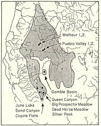
Figure 1 Map of the geographic range of the sagebrush least chipmunk, Tamias minimus scrutator, showing the locations of the populations sampled in Oregon, California, and Nevada.
Table 1 Estimates of genic variability at 27 presumptive allozyme loci in Tamias minimus scrutator. Standard errors are in parentheses for the mean heterozygosity (H) and average number of alleles (A). Percent polymorphic loci (P) is estimated for both the 0.01 and the 0.05 criteria (= frequency of the alternative allele).
| Population | n | H | A | P(0.01) | P(0.05) |
|---|---|---|---|---|---|
| Malheur 1 (MO1) | 18 | 8.42 (.02) | 1.70 (.26) | 33.33 | 29.63 |
| Malheur 2 (MO2) | 26 | 10.36 (.01) | 1.89 (.26) | 48.15 | 29.63 |
| Pueblo Valley 1 (PV1) | 23 | 9.16 (.01) | 1.89 (.37) | 37.04 | 22.22 |
| Pueblo Valley 2 (PV2) | 29 | 9.70 (.01) | 1.96 (.30) | 48.15 | 22.22 |
| Gamble Basin (GB) | 14 | 9.55 (.01) | 1.63 (.23) | 29.63 | 22.22 |
| June Lake (JL) | 25 | 9.79 (.01) | 1.81 (.27) | 44.45 | 33.33 |
| Sand Canyon (SC) | 32 | 10.78 (.01) | 1.78 (.32) | 33.33 | 25.93 |
| Coyote Flats (CO) | 22 | 9.40 (.01) | 1.59 (.25) | 33.33 | 22.22 |
| Queen Canyon (QC) | 17 | 9.41 (.01) | 1.59 (.24) | 29.63 | 22.22 |
| Big Prospector Meadow (BP) | 33 | 10.05 (.01) | 1.85 (.29) | 40.74 | 25.93 |
| Silver Peak (SP) | 18 | 10.00 (.02) | 1.74 (.27) | 37.04 | 29.63 |
| Dead Horse Meadow (DH) | 22 | 10.76 (.01) | 1.56 (.21) | 29.63 | 25.93 |
| Mean | 23.25 | 9.87 | 1.75 | 37.04 | 25.93 |
Data collection and management. Collection methods included Sherman livetraps (H. B. Sherman Co., Tallahassee, Florida, USA), Museum Special snap-traps, and shotgun. A total of 280 individuals were collected from the target 12 populations. An additional 32 specimens were collected within the range of T. m. scrutator, but only one or a few from each site so they did not constitute a population-level sample. Analyses and comparisons of populations used the 280 individuals from the 12 populations, but all 312 specimens were used for pooled analyses. Species identifications were based on morphology and geography and our analyses (see Results) confirmed all specimens were T. minimus. We assigned them as T. m. scrutator based on the geographic distribution of the subspecies. Skulls were collected from all the animals captured and post-cranial skeletons and skins were collected from some of the animals. There was variation in sample sizes among the characters measured due to damage from birdshot. Tissue samples (liver, heart and kidney, and blood) were frozen at -70°C for later processing.
Chipmunks were measured for 27 genetic (Supplemental Table 3), 50 morphological (Supplemental Table 4), and 11 lateral pairs of morphological cranial variants (to assess asymmetry; Supplemental Table 5). Sex was determined for all individuals, and they were assigned to one of seven age categories based on tooth wear and reproductive condition (Smith 1977). Sample sizes ranged from n = 14 (GB) to n = 33 (BP)
All individuals were analyzed for a standard set of 27 presumptive allozyme loci using established electrophoretic techniques (Selander et al. 1971) at the Museum of Vertebrate Zoology, University of California, Berkeley. Although not generally used in contemporary research, assessing allozyme alleles (the various forms of enzymes coded for by a single locus) was a useful method for characterizing genetic diversity prior to the development of genetic sequencing methods. Fifty morphological characters were measured (Supplemental Table 4). Four were external characters measured to the nearest mm. The remaining 20 skull and 26 skeletal characters were measured to the nearest 0.05 mm with dial calipers. Eleven paired sets of lateral epigenetic cranial threshold variants (hereafter lateral variants; Supplemental Table 5) were identified and tallied on 312 individuals (170 males, 142 females). These variants were scored as present (+) or absent (-).
Analyses. We assessed genetic variation within and among populations using goodness-of-fit statistics (Sokal and Rohlf 1969) and Wright’s F-statistics calculated across all alleles (Wright 1978) with their significance calculated using the procedure described in Eanes and Koehn (1978). All populations were tested for Hardy-Weinberg proportions using Levene’s (1949) corrections for small sample sizes in the estimation of expected genotype frequencies. Mean heterozygosity (H) by the direct count method, average number of alleles per locus (A), and percent polymorphic loci (P) were calculated for each population.
All morphological characters exhibited considerable sex-by-age interaction when combined over all populations. We attempted to diminish the influence of sexual dimorphism on the variation in characters and eliminate the potential bias due to variation in age distributions (see Baccus 1986). We calculated one-way analysis of variance (ANOVA) and t-tests for each character measured across the 12 populations and between sexes and age categories. A multiple range test using the Student-Newman-Keuls procedure was also used to assess trends in the means of the characters across populations. We calculated univariate comparisons of differences between populations for the external and skull characters and the skeletal characters using t-tests. Additionally, morphological variation was quantified for each population separately as a multivariate coefficient of variation (CVn) following the procedure of Van Valen (1974). CVn is independent of the number of variables used and so is numerically comparable to the univariate CV.
To compare the frequencies of the lateral variants among the 12 populations, we used a test of independence using the G-statistic. We calculated a sums-of-squares simultaneous-test-procedure (SS-STP) for characters with significant G-tests. We assessed the asymmetry measures for directional asymmetry using the Student’s t-test for paired comparisons, and for antisymmetry using a chi-square test for departures from normality (Soulé 1967). Additionally, the data were analyzed using Kendall’s coefficient of concordance, W, to determine if the level of fluctuating asymmetry is similar across all characters measured in the populations (Siegel 1956).
Relationships among populations within and between regions and within and between elevations were compared with geographic distances between populations. Genotype and allele frequencies were calculated for each population and for each region, each elevation, and the subspecies. Genetic distance measures were calculated using Nei’s (1978) genetic identity (I) and Roger’s (1972) genetic distance (S). We tested correlations between populations and elevation with a G-test of heterogeneity using allele frequencies. ANOVA was used to compare the frequency of the common alleles across populations and between regions and between elevations. We used Spearman’s rank correlation to determine any north-south or east-west clinal tendencies.
To evaluate the influence of geography on morphological differences among populations, we employed two separate distance indices. The first was Mahalanobis D2 (Reyment 1961; Gould and Johnston 1972). The mean of a character was substituted for missing values for that character in an individual. Mahalanobis D2 is highly affected by the sign and degree of correlation between the characters used. However, a major advantage of using Mahalanobis D2 is that it accounts for variation within populations. The significance of differences between population samples was determined by a multivariate analysis of variance using the BMDP(3D) program (BMDP Statistical Software, Inc., Los Angeles, California, USA).
The second morphological distance index we used was Lidicker’s Σd (Lidicker 1962). This index uses the differences between means of the characters divided by the minimum significant difference (msd), such that only mean differences greater than the amount that might be due to chance are treated as real differences. We used the estimate of msd equivalent to 2(SEx)1 + 2(SEx)2. This yields a conservative estimate with confidence limits usually well in excess of 95% (Lidicker 1962). The ratio of the difference between means for one character and the msd yields dimensionless numbers d1, d2, ..., dn for successive characters. Adding these pure numbers gives an estimate of total differentiation between a pair of samples in the characters studied (Σd). This index was modified slightly from Lidicker (1962) by including all characters, not just the ones with means greater than the msd. A given amount of differentiation between two samples in close geographic proximity has more biological significance than the same amount of differentiation between a geographically distant pair of samples. Lidicker (1962) suggested compensating for this by dividing the total differentiation by the distance between the two samples. We used indirect distances measured using presumed paths of gene flow between populations (Supplemental Table 2). This yields the Index of Differentiation (ID) representing the proportion of significant change that occurs between the two samples per kilometer. If distance is kept constant, ID will tend to increase as gene flow is reduced (Lidicker 1962).
We conducted a discriminant function analysis to visualize patterns of geographic variation across the 12 populations. We constructed phenograms from the genetic distance measures using Roger´s S and for the cranial dataset using Mahalanobis D2 values and Lidicker’s Σd values. Divergence measures of the 12 populations based on the asymmetry estimates were calculated following Grewal (1962). Correlations (Sokal and Rohlf 1969) were calculated between all the biological distance measures (Nei’s I and Roger’s S; Mahalanobis D2 and Lidicker’s Σd; asymmetric distinctiveness) and the geographic distance to determine the degree of concordance between the measures.
Results
Genetic variation within and among populations. The two Malheur (MO1, MO2) sites and the two Pueblo Valley sites (PV1, PV2) were first thought to be two populations (Malheur and Pueblo Valley). However, electrophoretic data at four loci (ALB-2, ADA, P-LGG, P-LA) revealed a Wahlund effect, therefore these two areas were each subdivided into two populations (MO1 and MO2, PV1 and PV2) such that each population had a sample size of at least 18 individuals captured within 0.75 miles (1.2 kilometers) of one another. The subdivided populations exhibited Hardy-Weinberg proportions. Because of the subdivisions and the spatial constraints placed on the “new” populations, 19 individuals from Malheur and nine individuals from Pueblo Valley were excluded from the population analyses but were included in analyses for the whole subspecies.
Of 27 presumptive loci, nine loci were slightly polymorphic, and four were highly polymorphic. Mean heterozygosities (H) ranged from 8.42 % at MOl to 10.78 % at SC and 9.86 % for the subspecies. The average number of alleles per locus (A) and percent polymorphic loci (P) were similar across populations (Table 1). Two criteria, 0.01 and 0.05 minimum frequency of alternate alleles, have been suggested for evaluating the polymorphism of a locus (Ayala et al. 1972; Nevo et al. 1974). Using the 0.01 criterion, virtually all rare alleles contributed to the values of P. Therefore, we used the values of P with the 0.05 criterion as it is much less affected by sample size. All values fell within two standard deviations of the mean and hence are considered to reflect a single statistical population. Across 170 comparisons of genotype, only three indicated a significant deviation from Hardy-Weinberg expectations: MO1 and SP at the ALB-2 locus and PV1 at the P-LA locus. With the large number of tests conducted, one would expect occasional (eight in this case) spurious differences to be found.
Table 2 Distribution of unique alleles across populations and loci. Total number of alleles at each locus are in parentheses. Populations that are not listed (SC, CO, QC, BP, SP, DH) had no unique alleles.
| Sample size | # Unique alleles | Loci w/unique alleles | % Individuals w/allele | % Individuals w/ a unique allele | |
|---|---|---|---|---|---|
| MO1 | 18 | 1 | ALB-2 (13) | 5.6 | 5.6 |
| MO2 | 26 | 2 | IDH-1 (4) | 3.8 | 7.7 |
| CK-3 (3) | 3.8 | ||||
| PV1 | 23 | 1 | LDH-1 ( 2) | 4.3 | 4.3 |
| PV2 | 29 | 1 | ALB-1 ( 2) | 3.4 | 3.4 |
| PV* | 1 | 1 | CK-2 ( 3) | ---- | ---- |
| GB | 14 | 3 | P-LGG (4) | 2.86 | 7.5 |
| MPI (3) | 0.71 | ||||
| 6-PGD (2) | 0.71 | ||||
| JL | 25 | 3 | IDH-1 (4) | 0.40 | 12.0 |
| IDH-1 (4) | 0.80 | ||||
| ACON1 (2) | 0.40 |
*from one individual removed from the detailed population analyses due to subdivision of the Pueblo Valley sample into two populations.
Geographic and elevational patterns in genetic variation. There was no pattern in any of the three indices (P, H, A) that could be construed as regional or elevational. However, there were no unique alleles found in populations located south of the 37° 30’ N parallel, suggesting some geographic role for shaping population variation. Generally, the ability to detect unique alleles increases with sample size. However, the two trapping localities (BP and SC) with the largest sample sizes contained no unique alleles, and the trapping locality with the lowest sample size (GB) had the largest proportion of individuals exhibiting a unique allele (35.7 %, Table 2). For the other four of the southernmost populations, the number of individuals with a unique allele ranged from 3.4 to 12.0 %. Measures of genetic distance (Roger’s S) and identity (Nei’s I) had similar patterns (Supplemental Table 6). The CO population had the largest average genetic distance using Roger’s S and the least average genetic identity using Nei’s I. A phenogram constructed from the values of Roger’s S between populations also showed CO as the most different (Figure 2). This phenogram also shows MO2 as being quite different from the other low-elevation populations and the other northern populations.

Figure 2 Phenogram from the cluster analysis using an unweighted pair-group method of the genetic distance estimated using Roger’s S.
The patterns of genetic differentiation between populations were not consistent across loci. Regional (i. e., grouping populations by mountain ranges) heterogeneity was found in two of the 13 heteroallelic loci. The White Mountains population samples (BP, SP, DH, QC) were significantly different (P < 0.05 and P < 0.01 for αGPD and SDH, respectively) from the Sierra Nevada population samples (CO, JL, SC). Spearman’s Rank correlation revealed a relationship between common allele frequency and longitude (P < 0.05) for SDH, supporting an east-west pattern differentiating the Sierra Nevada and White Mountains.
Wright’s FPT (heterogeneity among populations), FRT (heterogeneity among regions), and FPR (heterogeneity among populations within regions) are in Table 3. The populations were divided into four regions based on geographic proximity: Oregon (MO1, MO2, PV1, PV2), Stillwater Mountains (GB), Sierra Nevada (JL, SC, CO), and White Mountains (QC, BP, SP, DH). For 16 of the 21 loci, the values of FPR exceeded those of FRT indicating more variation among populations within regions than between regions. The loci that were exceptions to the pattern (SDH, 6-PGD, MPI, NP, CK-2) showed significant FRT values.
Table 3 Summary of FPT, a measure of among population variance; FPR, a measure of among population variance within regions; and FRT, a measure of among region variance in allele frequency for electrophoretic loci in the sagebrush least chipmunk.
| Locus | FPR | FRT | FPT |
|---|---|---|---|
| αGPD | 0.0674 | 0.0469*** | 0.1111*** |
| ADA | 0.0561 | 0.0358*** | 0.0899*** |
| PLA | 0.0521 | 0.0387*** | 0.0888*** |
| PLGG | 0.0377 | 0.0288** | 0.0654*** |
| ALB-2 | 0.0410 | 0.0214** | 0.0615*** |
| MPI | 0.0209 | 0.0374*** | 0.0575** |
| SDH | 0.0035 | 0.0522*** | 0.0555** |
| PGI | 0.0367 | 0.0170* | 0.0531** |
| CK-2 | 0.0111 | 0.0410*** | 0.0516** |
| IDH-1 | 0.0323 | 0.0133 | 0.0452* |
| CK-3 | 0.0216 | 0.0207* | 0.0419* |
| GOT-1 | 0.0217 | 0.0171* | 0.0384* |
| PGM | 0.0214 | 0.0136 | 0.0347 |
| 6PGD | 0.0061 | 0.0272** | 0.0331 |
| MDH-2 | 0.0245 | 0.0065 | 0.0308 |
| NP | 0.0053 | 0.0150* | 0.0202 |
| GDA | 0.0157 | 0.0037 | 0.0193 |
| LDH-1 | 0.0149 | 0.0040 | 0.0188 |
| ACON1 | 0.0117 | 0.0053 | 0.0169 |
| ALB-1 | 0.0216 | 0.0032 | 0.0158 |
| IDH-2 | 0.0103 | 0.0035 | 0.0138 |
| Mean | 0.0249 | 0.0215** | 0.0459* |
* P<0.05, ** P<0.01, *** P<0.001
Eight of the 13 polymorphic loci showed elevational heterogeneity (G-test of independence) without any geographic distance correlations or heterogeneity within elevations. The high-elevation populations exhibited no within-elevational heterogeneity with the exception of CO (also peripheral). Elevational heterogeneity (observation of a single allele in samples from similar elevations, but different from alleles at other elevations) was found for the CK-3 locus (P < 0.001), the PGM locus (P < 0.05), and the MDH-2 locus (P < 0.05) at mid and/or high elevations and the GOT-1 locus (P < 0.05) at low elevations. The mid-elevation JL, SC, and DH populations exhibited the greatest degree of polymorphism, while the low-elevation samples had the lowest degree of polymorphism for the CK-2 locus (P < 0.001) and the PGI locus (P < 0.01). A slight cline was exhibited by the IDH-1 locus (P < 0.05) with the high-elevation samples exhibiting the greatest degree of polymorphism and the low-elevation samples the lowest degree of polymorphism. We also found a latitudinal correlation in the IDH-1 locus (Spearman’s Rank correlation, P < 0.05). The highly polymorphic P-LA locus exhibited only elevational heterogeneity (P < 0.001), even when the CO sample was removed from consideration. The CO sample contained only two of the five alleles present in all other populations plus a reversal of the dominant allele. The highly polymorphic P-LGG locus also exhibited elevational heterogeneity, but the heterogeneity between elevations was due mainly to the low elevations possessing a greater frequency of alternate alleles (P < 0.01). The fact that the low-elevation populations were also geographically distant complicates the pattern of elevational heterogeneity. There was a slight degree of heterogeneity (P < 0.05) between the mid- and high-elevation samples, but it disappears when GB, which is geographically distant, is removed from consideration. The Sierra Nevada and White Mountains samples are homogeneous with respect to this locus.

Figure 3 Phenogram from the cluster analysis using the unweighted pair-group method for population distances based on Mahalanobis D2 from the cranial dataset.
Supplemental Table 7 gives the values for FPE (measures heterogeneity among populations within elevations), FET (measures heterogeneity among elevations), and FPT (measure the overall degree of heterogeneity among populations) for the loci that were heteroallelic in the Sierra Nevada and White Mountains populations. Restricting the analysis to these two areas eliminated biases due to region. The Sierra Nevada and White Mountains are adjacent and parallel mountain chains containing populations that were classified as either mid- or high-elevation. These data indicated that genetic structuring did not follow an elevational pattern. Twelve of the 13 loci exhibited more variation among populations within elevations than between elevations. One locus (P-LA) had high within-elevation heterogeneity, likely due to the uniqueness of the CO population. When the CO sample was removed from consideration, G-tests showed no significant heterogeneity within low- and mid-elevation samples, and the heterogeneity within high-elevation samples disappeared.
Two of the highly polymorphic loci (ALB-2, ADA) were responsible for the Wahlund effects that necessitated a division of the Pueblo Valley and Malheur samples. The high degree of populational heterogeneity in the ALB-2 samples (P < 0.001) confounded any elevational heterogeneity that might be present. Among the low-elevation samples, PV1 and PV2 were significantly different (P < 0.001) from MO1 and MO2 while, within each area, there was homogeneity. All mid- and high-elevation populations were unique at these loci.
The ADA locus showed a pattern of elevational heterogeneity overlain with a pattern of latitudinal heterogeneity (Spearman’s Coefficient of Rank Correlation, P < 0.05). There was homogeneity among the low-elevation samples; however, they were significantly different from both the mid-elevation samples (P < 0.001) and the high-elevation samples (P < 0.001). There appears to be a break in continuity around the 37° 30’ N parallel among the mid-elevation samples, causing JL and GB to be grouped and SC and DH to be grouped even though these populations are not geographically close. Among the high-elevation populations, the break in continuity may occur around the 37° 20’ N parallel which would group the three White Mountains populations (QC, SP, BP) together leaving the CO population (in the Sierra Nevada) unique. Whether the latitudinal break is valid for the high-elevation populations or the populations are exhibiting regional heterogeneity could not be determined from this dataset.
Geographic and elevational patterns in morphological variation. Twenty-two of the 24 skin and skull characters (Table 4) and 12 of the 26 postcranial skeleton characters showed significant interpopulation variation (Supplemental Table 8). A sums of squares-simultaneous test procedure (SS-STP) across means of the characters in the cranial dataset with significant interpopulation variation showed no discernable trends across regions or elevation. However, the CO samples had the greatest mean value for 10 of the 24 characters; only 1.2 cases would be expected by chance alone. The BP sample had the greatest mean value for three characters. MO1, MO2, PV1, and PV2 (all low-elevation samples) were grouped together or separated by only SC, JL, or GB in eight characters. The four southernmost populations (BP, SP, DH, CO) were grouped together for 10 characters. For 19 characters, there were same-elevation, same-geographic area clusters (MOI-MO2, PVI-PV2, JL-SC, QC-BP, BP-SP).
Table 4 Multiple range tests (Student Newman-Keuls procedure) for means of the external and cranial morphological characters (22 of 24) exhibiting significant interpopulation variance after adjustments for sex and age variation for the 12 populations of Tamias minimus scrutator. Interpopulation F-values (ANOVA) and significance are below character abbreviations.
| 1. BDL | MO1 | MO2 | QC | GB | BP | SP | SC | JL | PV1 | DH | CO | PV2 | ||
| 4.9*** | |--------------------------------------------------------------------------------| | |||||||||||||
| |--------------------------------------------------------------------------------| | ||||||||||||||
| |-------------------------------------------------------------------------------------------| | ||||||||||||||
| |----------------------------------------------------------------------| | ||||||||||||||
| 2. TAL | SP | DH | GB | BP | QC | CO | MO1 | JL | SC | PV2 | MO2 | PV1 | ||
| 2.2* | |---------------------------------------------------------------------------------------------| | |||||||||||||
| |-------------------------------------------------------------------------------------------------------------------| | ||||||||||||||
| 3. HFL | SP | SC | DH | PV2 | JL | GB | PV1 | BP | MO1 | MO2 | QC | CO | ||
| 3.7*** | |---------------------------------------------------------------------------------------------| | |||||||||||||
| |--------------------------------------------------------------------------------------------------------| | ||||||||||||||
| |----------------------------------------------------------------------| | ||||||||||||||
| 4. EAR | BP | MO1 | SP | JL | PV2 | GB | CO | PV1 | MO2 | DH | QC | SC | ||
| 4.2*** | |--------------------------------------------------------------------------------------------------------------------| | |||||||||||||
| |------------| | ||||||||||||||
| 5. LNA | QC | MO2 | JL | MO1 | GB | CO | SC | PV2 | PV1 | SP | BP | DH | ||
| 3.0*** | |------------------------------------------------------------------------------------------------------------------------------| | |||||||||||||
| 7. GSL | MO2 | MO1 | QC | JL | PV1 | SP | DH | SC | PV2 | GB | BP | COI | ||
| 3.2*** | |--------------------------------------------------------------------------------------------------------| | |||||||||||||
| |--------------------------------------------------------------------------------------------------------------------| | ||||||||||||||
| 8. BSL | MO2 | SC | MO1 | DH | QC | JL | PV1 | SP | PV2 | CO | BP | GB | ||
| 3.0*** | |---------------------------------------------------------------------| | |||||||||||||
| |--------------------------------------------------------------------------------------------------------------------| | ||||||||||||||
| 9. TRL | QC | MO2 | JL | GB | SC | SP | BP | PV1 | MO1 | CO | DH | PV2 | ||
| 2.5** | |-------------------------------------------------------------------------------------------------------------------| | |||||||||||||
| |--------------------------------------------------------------------------------------------| | ||||||||||||||
| 1.9* | |-------------------------------------------------------------------------------------------------------------------| | |||||||||||||
| |-------------------------------------------------------------------------------------------------------| | ||||||||||||||
| 13. MAL | QC | MO2 | MO1 | SC | JL | GB | PV1 | PV2 | DH | BP | SP | CO | ||
| 2.8** | |-------------------------------------------------------------------------------------------------------------------| | |||||||||||||
| |-------------------------------------------------------------------------------------------------------| | ||||||||||||||
| 14. MAD | SC | QC | JL | PV2 | MO2 | MO1 | PV1 | DH | SP | GB | BP | CO | ||
| 3.8*** | |-------------------------------------------------------------------------------------------------------| | |||||||||||||
| |------------------------------------------------------------------------------------------------------------------| | ||||||||||||||
| 15. APW | SC | MO2 | MO1 | PV2 | DH | PV1 | JL | CO | QC | SP | GB | BP | ||
| 4.6*** | |----------------------------------| | |||||||||||||
| |-------------------------------------------------------------------------------------------------------| | ||||||||||||||
| |-------------------------------------------------------------------------------------------------------| | ||||||||||||||
| 16. ROD | MO2 | MO1 | QC | SC | PV1 | PV2 | GB | JL | DH | SP | CO | BP | ||
| 5.8*** | |----------------------------------------------| | |||||||||||||
| |--------------------------------------------------------------------------------| | ||||||||||||||
| |-------------------------------------------------------------------| | ||||||||||||||
| 17. CRD | MO1 | GB | JL | BP | PV1 | MO2 | SP | QC | PV2 | SC | CO | DH | ||
| 3.2*** | |-----------------------------------------------------------------------------------------| | |||||||||||||
| |------------------------------------------------------------------------------------------------------------------| | ||||||||||||||
| 18.SKD | QC | GB | PV1 | JL | MO1 | MO2 | PV2 | SP | BP | CO | SC | DH | ||
| 4.0*** | |------------------------------------------------------------------------------------------------------------------| | |||||||||||||
| |-----------| | ||||||||||||||
| 19. ILW | MO2 | SC | PV1 | PV2 | MO1 | JL | QC | GB | SP | DH | CO | BP | ||
| 4.5*** | |--------------------------------------------------------------------------------------------| | |||||||||||||
| |--------------------------------------------------------------------------------------------| | ||||||||||||||
| |--------------------------------------------------------------------------------------------| | ||||||||||||||
| |----------------------------------------------------------| | ||||||||||||||
| 20. LOW | SC | SP | MO2 | JL | PV2 | GB | QC | BP | MO1 | PV1 | DH | CO | ||
| 2.8** | |-------------------------------------------------------------------------------------------------------------------| | |||||||||||||
| |--------------------------------------------------------------------------------| | ||||||||||||||
| 22. IMW | QC | MO1 | JL | PV2 | MO2 | GB | SP | BP | DH | SC | PV1 | CO | ||
| 3.9*** | |------------------------------------------------------------------------------------------------------| | |||||||||||||
| |---------------------------------------------------------------------------------------------------------| | ||||||||||||||
| |----------------------------------| | ||||||||||||||
| 23. BOW | JL | SC | GB | MO2 | MO1 | PV1 | PV2 | QC | DH | BP | SP | CO | ||
| 2.4** | |------------------------------------------------------------------------------------------------------------------| | |||||||||||||
| |---------------------------------------------------------------------------------------------------------| | ||||||||||||||
| 24. CWO | QC | MO1 | JL | MO2 | PV1 | PV2 | SC | SP | DH | BP | GB | CO | ||
| 2.8** | |-------------------------------------------------------------------------------------------------------------------| | |||||||||||||
| |---------------------------------------------------------------------------------------------------------| | ||||||||||||||
* P < 0.05; ** P < 0.01; *** P < 0.001
1. BDL = Body length; 2. TAL = Tail length; 3. HFL- = Hind Foot length; 4. EAR = Ear length; 5. LNA = length of Nasals; 7. GSL = Greater Skull length; 8. BS = Basal Skull length; 9. TRL = Tooth Row length; 10. IFL = Incisive Foramen length; 13. MAL = Mandible length; 14. MAD = Mandible Depth; 15. APW = Angular Process width; 16. ROD = Rostral Depth; 17. CRD = Cranial Depth; 18. SKD = Skull Depth; 19. ILW = Interlacrimal width; 20. LOW = Least Orbital width; 21. GZW = Greatest Zygomatic width; 22. IMW = Intermaxillary width; 23. BOW = Basioccipital width; 24. CWO = Cranial width Obliquely.
For the cranial dataset, the MO1, CO, and BP samples had the highest multivariate CVn and the SP and PV1 samples had the lowest values. Overall, the postcranial skeletal characters had higher CVn than the skin and skull characters. The CVn had no discernable geographic trends.
The morphological distance indices, Mahalanobis D2 along with F-values and a modification of Lidicker’s Σd along with an Index of Differentiation, recovered similar distances among populations, with some notable exceptions (Supplemental Table 9). SC was significantly different from all other populations and CO was significantly different from all but two (SP and DH, the other southernmost populations). JL exhibited significant differences from five other populations, with no apparent pattern to the distribution of differences. This population, centrally located (both geographically and elevationally), had one of the smallest values for both Mahalanobis D2 and Lidicker’s Σd. GB, the most geographically isolated population, had the highest Mahalanobis D2 value but one of the smallest for Lidicker’s Σd. GB also had the smallest average Lidicker’s ID value, which is not unexpected given that GB is geographically distant from the other sampled populations. Overall, a comparison of Lidicker’s ID against geographic distance between the populations yielded a significant negative correlation (r = -0.44, P < 0.001), indicating that within the subspecies, differentiation among populations did not consistently increase with the distance between them. For the cranial dataset, there was no correlation between Lidicker’s Σd and geographic distance (r = 0.15) nor between Mahalanobis D2 and geographic distance (r = 0.02).
A phenogram constructed from the Mahalanobis D2 values for the cranial dataset (Figure 3) indicated GB was the most different and CO and SP clustered closely together. DH was grouped with PV1 and PV2, and the rest of the populations formed a fourth cluster. The phenogram constructed from the modified Lidicker’s Σd values for the cranial dataset (Figure 4) showed a clustering of the southernmost populations (CO, SP, DH, BP), but with JL and QC associating with the northern populations; SC was intermediate.
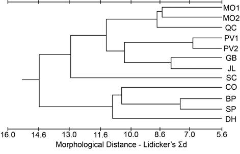
Figure 4 Phenogram from the cluster analysis using the unweighted pair-group method for population distances based on Lidicker’s Σd from the cranial dataset.
Geographic and elevational patterns in asymmetry. Divergence of the 12 populations was calculated based on the frequencies of asymmetry (Supplemental Table 10). None of the populations was significantly different from any other population. Asymmetry between the right and left sides of the cranium was recorded for 11 bilateral variants (22 total, 11 characters on each side). The JL, SC, and DH samples had the highest level of asymmetry and CO had the lowest level of asymmetry when averaged over all pairs of lateral variants. Two pairs of lateral variants (FOD and OFD) exhibited significant interpopulation heterogeneity (G = 22.004, P < 0.05; and G = 24.256, P < 0.05; respectively). For the FOD lateral variants, the interpopulation heterogeneity resulted from a large frequency of asymmetry in JL. Grouping populations by elevation indicated significant (G = 13.530, P < 0.01) between-elevation heterogeneity and no significant within-elevation heterogeneity. For the OFD lateral variants, the heterogeneity can be assigned to the White Mountains populations where the high-elevation populations (QC, BP, SP) were significantly different (G = 9.671, P < 0.05) from the mid-elevation DH population. The White Mountains high-elevation populations were also significantly different (G = 12.469, P < 0.01) from the other high-elevation population (CO). None of the other asymmetry estimates had interpopulation variation, sexual dimorphism, or heterogeneity between age categories. Tests of antisymmetry indicated that no characters we measured had a probability that the variant would be seen more often on one side than the other. All other asymmetries (except for a slight directional asymmetry in the JL population) are assumed to be fluctuating asymmetry, which are the minor departures from complete bilateral symmetry which have no known adaptive advantage. Testing the lateral variants for similarities within populations using Kendall’s test for concordance yielded a non-significant value (W = 0.105, P > 0.50) indicating the characters form a normal distribution around a mean, supporting the conclusion that they show fluctuating asymmetry. A phenogram based on asymmetric divergences yielded no clear geographic patterns (Figure 5).
Comparisons of genetic, morphological, and geographic patterns. The two morphological distances (Mahalanobis D2 and Lidicker’s Σd) were correlated with the two genetic distance measures (Roger’s S and Nei’s I; Table 5). Lidicker’s Σd was positively correlated with Roger’s S and negatively correlated with Nei’s I. Mahalanobis D2 was negatively correlated with Roger’s S and positively correlated with Nei’s I (though not significantly). Roger’s S was the only biological distance measure positively and significantly correlated with geographic distance. Assuming that longer geographic distances tend to distort the accuracy of the biological distance measures, we calculated correlations using only samples located less than 112 km from one another, as measured on a map. Roger’s S and geographic distance were no longer correlated in the reduced dataset. Lidicker’s Σd and Mahalanobis D2 were no longer correlated with either Roger’s S or Nei’s I. Further restriction of the dataset to just the White Mountains and Sierra Nevada populations yielded a significant correlation between Mahalanobis D2 and the asymmetry divergence measures. Roger’s S and Nei’s I were still negatively correlated, but the other correlations were no longer significant.
Table 5 Matrix of inter-correlations of biological and geographic distances. The first row of each measurement is correlation coefficients using the complete dataset (n = 66); second row is correlation coefficients using only comparisons between populations less than 1 ○ latitude (<112 km) apart (n = 27); third row is correlation coefficients using only comparisons between population in the White Mountains and Sierra Nevada (n = 21).
| Nei’s I | Roger’s S | MAH D2 | LID Σd | ASYM | DIRECT GEO | |
|---|---|---|---|---|---|---|
| Roger’s S | -0.804*** | |||||
| -0.922*** | ||||||
| -0.937*** | ||||||
| Mahalanobis D2 | 0.194 | -0.260* | ||||
| 0.071 | -0.157 | |||||
| 0.047 | -0.108 | |||||
| Lidicker’s Σd | -0.329** | 0.320** | 0.037 | |||
| -0.309 | 0.321 | 0.309 | ||||
| -0.210 | 0.168 | 0.341 | ||||
| Asymmetry | -0.040 | 0.060 | 0.093 | -0.218 | ||
| -0.226 | 0.243 | 0.325 | 0.036 | |||
| -0.108 | 0.093 | 0.445* | -0.044 | |||
| Direct Geographic | -0.098 | 0.304* | 0.028 | 0.155 | -0.202 | |
| -0.047 | 0.043 | 0.196 | 0.286 | -0.066 | ||
| -0.14 | 0.191 | -0.052 | 0.272 | 0.071 | ||
| Indirect Geographic | -0.127 | 0.333** | 0.084 | 0.149 | -0.183 | 0.925*** |
| -0.396* | 0.354 | 0.020 | 0.287 | -0.074 | 0.422* | |
| -0.368 | 0.318 | -0.100 | 0.142 | -0.183 | 0.347* |
* P<0.05; ** P<0.01; *** P<0.001
Discussion
Our assessment of variation in sagebrush least chipmunk populations demonstrated substantial differentiation among populations across genetic and morphological traits. The most conspicuous observation from the electrophoretic dataset is that all populations were unique and the unique factors varied among populations. As with the electrophoretic data, the morphological measures for the 12 populations exhibited a considerable degree of interpopulation differentiation. Asymmetries of lateral variants also had attributes of population-level interest. Overall, we found a lack of correlation between geographic distance and differentiation (as measured by the biological distances), supporting T. m. scrutator as a single subspecies.
If random genetic drift is the overriding influence in the differentiation of populations, then we expect to find a random pattern of variation between populations. Our findings for the fixation indices for the four major regions (a measure of genetic drift) indicated more differentiation within regions and elevations than between regions or elevations. For example, the two Malheur (MO1, MO2) and the two Pueblo Valley (PV1, PV2) populations exhibited a Wahlund effect in the heterozygosity measures. A random pattern of variation was also seen for six morphological characters. Taken together, these results suggest a considerable role for genetic drift in driving population structure for T. m. scrutator.

Figure 5 Phenogram from the cluster analysis using the unweighted pair-group method for population distances based on asymmetry divergence taken from the cranial dataset.
Population structure. We found that geographic distance and genetic drift are the most likely explanations for how variation is structured across populations but cannot rule out contributions from selection associated with elevation in some populations. Most population differences in the genetic dataset can parsimoniously be attributed to random genetic drift. The fixation indices (Table 3) are essentially measures of genetic drift, probably due to differences in the founding populations (Wright 1978). Reduced levels of gene flow would enhance any population differences originating by genetic drift or selection, and would also tend to maintain differences between the populations.
Population variation potentially resulting from selection at different elevations was suggested by variation at seven genetic loci and one morphological character. We also found an elevational trend for population variation in asymmetry. Elevation was chosen for detecting selection as it has been shown to generate differences in other species, probably due to climatic characteristics (Dunmire 1960; Asdell 1964; States 1976; Baccus et al. 1980). Assessment of elevational patterns was complicated by the fact that the populations grouped within the same elevation also tended to be within the same geographic region. However, focusing on just two regions (White Mountains and Sierra Nevada) and two elevations revealed elevational heterogeneity with no regional heterogeneity in four loci. This illustrates that selection may be playing a role in the genetic structuring at these particular loci or at loci linked to them. The case is particularly strong for the CK-2 locus as it exhibited little heterogeneity within elevations. Sagebrush least chipmunks would serve as a good model to compare to the elevational adaptations found in other mammals, such as deer mice (Peromyscus maniculatus; Storz et al. 2019).
The most prevalent pattern emerging from the morphological dataset is a separation of populations based on latitude irrespective of elevation. Fully half of the 20 characters with a significant F-ratio had little variation within populations grouped according to latitude (Table 4). Populations below the 37° 30’ parallel (CO, BP, SP, DH) formed a subset for 10 characters as did populations located between 37° 30’ and 41° latitude (JL, QC, GB) and the populations above the 41° parallel (MOl, MO2, PV1, PV2). If another division is added at the 43° parallel (separating MOl and MO2 from PVI and PV2), five more characters (for a total of 75 % of the characters with significant F-ratios) conform to this pattern. The remaining 25 % of the morphological characters with significant interpopulation variation, as well as the occurrence of sexual dimorphism across populations in some of the characters, exhibited a random pattern of variation. This would be expected under the influence of genetic drift, which is further supported by our finding of no unique allozyme alleles south of the 37° 30’ parallel.
Peripheral populations. The peripheral populations (CO, BP, DH, SP) had mixed signals of population differentiation, with some traits supporting isolation (Figures 3, 4), but other approaches (Figures 2, 5) suggesting that periphery of the subspecies range is not a major factor partitioning variation among these populations. As there are no direct dispersal routes through sagebrush habitat between the CO (Sierra Nevada) population and the White Mountains populations (BP, DH, SP), if these peripheral populations were morphologically similar due to gene flow, they should also be similar to the other two Sierra Nevada populations (SC, JL) and the other White Mountains population (QC). This was not the case, as those other populations grouped with northern populations more than 350 km away (Figures 3 and 4). This pattern that cannot be explained by differentiation due to distance suggests genetic drift as a significant factor shaping the populations.
The paucity of rare alleles in the southern populations could be an indication of the marginality of these populations (although it may reflect historical biogeography). Central areas are thought to be more tolerant of alternate forms and also exhibit more genetic inertia while marginal areas maintain more intense selection limiting the number of phenotypes that are able to survive and reproduce. Chipmunks are adapted to utilize areas with harsh winters by hibernating intermittently, i. e., they make use of mild days to supplement winter stores. Marginality in a geographic sense may have a greater effect on allele frequencies. For example, the occurrence of only two of the five alleles of the P-LA locus, and the reversal of the common allele for both the P-LA and ADA loci were noted in peripheral populations. Our data also indicated isolated populations are more genetically distinct, supporting isolation having a greater impact on population structure than periphery. The GB population is by far the most distinct in regard to individuals sporting a unique allele, as well as in average morphological (Mahalanobis D2) divergence measures, and it appears to be the most geographically isolated of our samples. GB is a peninsular population (it can only receive migrants from one direction) due to incompatible habitats almost completely surrounding the Stillwater Mountains where it occurs.
Variation in population structure across markers. Genetic, morphological, and lateral variant traits did not have consistent signals. The morphological data even indicated different signals depending on how the data were analyzed. The large discrepancies between biological distance measures indicate that each may be measuring different characteristics of the phenome. For example, Mahalanobis distance and asymmetry divergences measure levels of variation among the populations accurately only over short geographic distances, whereas Lidicker’s distance measure along with the genetic distance measures (Roger’s and Nei’s) reflect larger-scale genetic affinities among the populations.
Additional considerations. Historically, the geographic range of sagebrush least chipmunks probably extended southward into what is presently the Mojave Desert and likely included the valley floor of what is present-day Owens Valley in California (however, see Grayson 1982). As the area became increasingly arid, the least chipmunk and its associated community retreated northward and to higher elevations, leaving the valley floors to more arid-adapted species. In extreme cases, populations became relatively isolated on islands or peninsulas connected by narrow straits of suitable habitat (Spaulding 1980).
Based on the assumption that isolated and/or peripheral populations with little gene flow should have lower levels of asymmetry than populations in central areas, the JL and DH populations, with the highest average level of asymmetry, should be the least isolated and, the CO population with the lowest average level of asymmetry should be the most isolated. Our electrophoretic data were consistent with the CO population as a peripheral isolate. The JL sample, as well as the DH and SC samples, are all mid-elevation samples located well within the species’ range and adjacent to areas of both higher and lower elevations. Hence, they may experience an influx of genes not well adapted to the mid-elevation environment. A higher level of asymmetry was expected for the non-peripheral ecologically marginal populations (QC, BP, SP), as they may experience maladaptive gene influx. However, these populations only grouped together in one of the lateral variant asymmetries (OFD), yielding lower asymmetry values for the grouping QC-BP-SP when compared to either their regional mate (DH) or their elevational mate (CO). There were no trends in the overall or average levels of asymmetry that corresponded to any of the regional (gene flow) or latitudinal (historical divergence time) trends, but there was an elevational (selective regime) trend. Removing the populations with a relatively high degree of isolation (GB, CO) leaves the mid-elevation samples with the highest levels of asymmetry as predicted, and the high-elevation samples with a median level. The low-elevation samples had the lowest levels of average asymmetry.
It is unlikely that the differences between the two Malheur populations and between the two Pueblo Valley populations can be attributed to selection. They are at similar elevations (implying similar climatic conditions) and in the same habitat type with similar terrains. Instead of selection, these chipmunks may have sufficiently low vagility that gene flow is incapable of overcoming stochastic differences among local populations. Limitation of gene flow would enhance the effects of any differential selection or drift (Wright 1948; Dobzhansky 1968). Examining the electrophoretic data as a complete unit, the populations show a similarity higher than would be expected for local populations of rodents (Avise 1976). So, even though there are real and striking differences between the populations, the overall similarities are high.
These data and results provide a valuable baseline for investigations of how population structure may have changed, or to investigate the impact of climate change on sagebrush least chipmunks. There is ample evidence that many mammal species, including chipmunks, are shifting distributions (Moritz et al. 2008) and are experiencing altered population dynamics and diversity (Rubidge et al. 2008) in response to climate change. Some isolated chipmunk populations in the Great Basin are genetically distinct and potentially threatened by habitat loss (Bell et al. 2021). Contemporary investigation of T. m. scrutator populations could gauge changes in population fragmentation and diversity, particularly in the peripheral and isolated populations that may warrant recognition as distinct population segments or may have experienced increased isolation and associated genetic drift. Additionally, genomic approaches could be used to test for variation in selection at different elevations, an important consideration for species that are anticipated to shift their elevational distributions in response to changing climate conditions.

