


 text new page (beta)
 English (pdf)
 Article in xml format
 Article references
 Send this article by e-mail
 Cited by SciELO
  Similars in
SciELO
Similars in
SciELO 
 Permalink
Introduction
Peromyscus furvus is an endemic Cricetid species from southeastern México that inhabits the temperate cloud and mixed forests from montane highlands and currently is considered as a monotypic species (Rogers and Skoy 2011; but see Ramírez-Pulido et al. 2014). Its current distribution ranges from southeastern San Luis Potosí, along the Sierra Madre Oriental, through the Faja Transvolcánica Mexicana and southward to the Sierra Norte de Oaxaca (Rogers and Skoy 2011). The species includes in synonymy (Musser 1964; Hall 1968; Huckaby 1980) Peromyscus latirostris (Dalquest 1950 - type locality Xilitla, San Luis Potosí) and P. angustirostris (Hall and Álvarez 1961 - type locality Zacualpan, Veracruz), as well as unassigned specimens from Puerto de la Soledad, Oaxaca.
Although P. furvus currently is considered a monotypic species (Rogers and Skoy 2011), several previous studies, under different epistemological and methodological approaches, have noted differences among its synonyms and assigned populations. Such differences include skull size (Musser 1964; Hall 1968; Martínez-Coronel et al. 1997; Ávila-Valle et al. 2012), allozymes (Harris and Rogers 1999), and mitochondrial genetic sequences (cytochrome-b gene, Harris et al. 2000, and ND3-ND4 genes, Ávila-Valle et al. 2012). In particular, genetic studies have added two distinct scenarios to the status of populations within P. furvus. One scenario (Harris et al. 2000) based on data from the Cytb gene is: a) that the southernmost populations from Puerto de la Soledad, Oaxaca genetically are distinct from others; and b) that the northernmost populations in Xilitla, San Luis Potosí are distinct from P. furvus proper. In the geographically intermediate zone, populations from Hidalgo, northern Veracruz and Puebla, historically attributed to angustirostris, appear separated from populations from central Veracruz (Xalapa, type locality of furvus) but are contained in the same basal clade
The second scenario, based on data from NAD3-ND4 genes (Ávila-Valle et al. 2012), suggests: a) that the most genetically distinctive populations are the northernmost ones from Xilitla, San Luis Potosí and Santa Inés, Querétaro (latirostris) and b) that populations from Hidalgo, Puebla, Veracruz, and Oaxaca are grouped together in a central-southern clade. This southern clade appears to contain three subclades: one from Mesa de la Yerba and Xico, Veracruz (furvus), a second from El Salto, Puebla (angustirostris), and a third containing populations from Puerto de la Soledad, Oaxaca and the remaining populations from Hidalgo, Puebla, and Veracruz, including the type locality of angustirostris. These scenarios lead to the following questions: how many different entities or distinctive genetic groups are included within the “monotypic” P. furvus? What is the level of genetic variation associated with the recognizable taxonomic units, e. g., species and subspecies? Do the specimens from the northern and southern ends of the distribution deserve specific recognition? What is the systematic and taxonomic status of the intermediate populations in Hidalgo, Puebla, and Veracruz?
Herein, the degree and level of divergence in populations from throughout the geographic range of P. furvus was assessed in order to understand if P. furvus consisted of one or more evolutionary and taxonomic entities. Our analyses included genetic (mitochondrial genes), morphogeometric (ventral shape of skull), and magnitude characters (centroid size of the latter and linear measurements for skull). Results from the genetic analyses are reported herein, whereas additional morphometric analyses will be presented in a separate manuscript. Additional genetic analyses were conducted to shed light into the complex relationships among populations of the intermediate geographic zone (Harris et al. 2000; Ávila-Valle et al. 2012).
Finally, Bradley et al. (2007) reported some uncertainty in the composition of the furvus species group within the genus Peromyscus. For example, P. furvus historically has been included in different species groups (e. g., mexicanus species group; Hooper 1968; Huckaby 1980) until it was assigned to its own group (Carleton 1989). However, the species composition within the furvus species group also has varied among authors (Carleton 1989; Wade et al. 1999; Musser and Carleton 2005). Herein, results from our analyses contribute to refine the composition of the furvus species group, in the light of the latest phylogenies provided for the genus (Bradley et al. 2007; Platt et al. 2015).
Materials and methods
Definition of groups. Populations from the geographic range of Peromyscus furvus were arranged into Operational Taxonomic Units (OTUs) according to their historical or current taxonomic designation and to their geographic provenance (Appendix 1, Figure 1). Hereafter, we refer to the OTUs of the Ingroup (IG) as Genetic Groups (GG1-5). GG1-3 with their taxonomic designations and their States of origin are: GG1 (latirostris, Pl) from San Luis Potosí and Querétaro; GG2 (angustirostris, Pa) from Hidalgo, Puebla, and Veracruz; and GG3 (furvus, Pf) from central Veracruz. The specimens with no formal designation include samples from two localities in Oaxaca, Puerto de la Soledad, referred to as GG4 (Oax18), and La Esperanza, GG5 (Oax19); however, GG5 samples lacked genetic data and were included only in morphometric analyses. We also selected five OTUs as Outgroups (OGs) based on evidence from recent phylogenies for peromyscines (Bradley et al. 2007; Platt et al. 2015). The three congeneric species include P. ochraventer (Poc) and P. melanocarpus (Pml), which have been associated with the furvus species group by Carleton (1989) and Musser and Carleton (2005), respectively, and P. mexicanus totontepecus (Pmt) from the closely related mexicanus group. Also, based on the aforementioned studies (Bradley et al. 2007; Platt et al. 2015), we included two additional species from different genera; Megadontomys cryophilus (Mcr), given its relative closeness to P. furvus, and Osgoodomys banderanus (Oba) as the most distant and possibly more conserved species (i. e., tentative root).
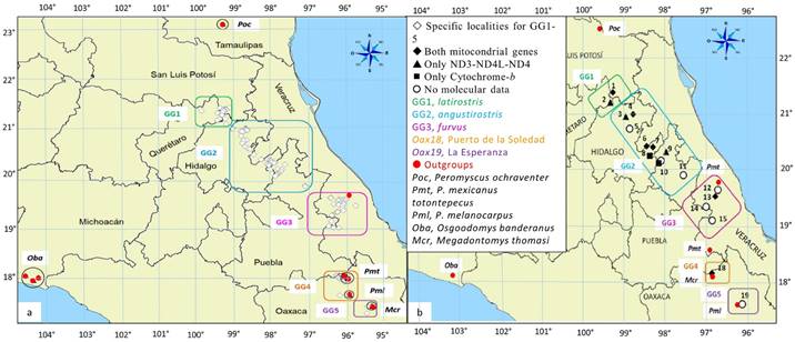
Figure 1 Geographical delimitation of the Genetic Groups (GG1-5) in the distribution of Peromyscus furvus used in this study as Ingroups (IGs), together with five outgroups (see legend); GG5 was included only in morphometric analyses. The map in (a) shows the location of specific localities that were pooled into group localities (numbers 1-19) in further analyses (b). See Appendix for details.
Molecular characters. Genetic sequences were downloaded, as complete as possible, from GenBank® (Genetic Sequence Database) for Cytochrome b gene (Cyt-b; IG n = 53, OG n = 13) and for three genes of the Nicotinamide Adenine Dinucelotide Hydride (NADH: ND3-ND4L-ND4; IG n = 57, OG n = 6). The sole exception was a sequence of NADH genes for Poc obtained from Wade et al. (1999). The sequences were aligned beginning at the start codon with the MEGA7 ClustalW option (Molecular Evolutionary Genetics Analysis, Ver. 7.0-7.2, Kumar et al. 2016) and truncated to similar lengths in all taxa. We analyzed 719 bases from the Cytb gene and 971 bases from the NADH genes (ND3, 306; ND4L, 293; ND4, 373; the tRNA-Arg interegion was eliminated, as it was unknown for Pml). Information about the geographic origin of sequences, GenBank accession numbers, and references appear in the Appendix.
Morphometric characters (continuous linear measurements). In our analyses of overall skull size, we included all OTUs (GG1-5 + five OGs). Herein, 233 specimens from 129 specific localities (SL) represented the IG, and 116 specimens from 11 SL represented the OG. We georeferenced all SLs using QGIS Wien (ver. 2.080-2.93) to project them onto a map (Figure 1A) and to pool the IG samples into 19 group localities (GLs), which in turn were assigned to GG1-5. We also used geographic coordinates of GLs to estimate the geographic distances (km) between every pair of GLs. Morphometric characters for analysis of overall skull size comprised 18 cranial measurements from adult specimens following Ávila-Valle et al. (2012; see figure 1:167 therein). Additional specimens were added to increase sample sizes in all OTUs (n ≥ 15, except for Mcr, n = 14). Appendix provides the geographical data, sample sizes, and museum designations.
Analyses of the ventral shape and size of the skull were based on only complete and undamaged skulls (listed in bold in the Appendix). We selected five structures from the ventral view of skull as morphogeometric characters. The details for the anatomical origin of the structures (and substructures contained in them), as well as the quantity and position of the landmarks and semilandmarks outlining each morphogeometric configuration, will be described elsewhere. We measured each skull with type 1 and 2 landmarks sensuBookstein (1991), taken from the literature (Myers et al. 1996; Cordeiro-Estreia et al. 2008; Grieco and Rizk 2010; Cordero and Epps 2012; Holmes et al. 2016), using utilities in the TPS series (Thin Plate Spline, Ver 2.31, TPS, available at https://life.bio.sunysb.edu/morph/ ...html; Rohlf 2015). In the examination of cranial contours, we followed Sheets et al. (2004) to adjust the semilandmarks. In the data matrix for morphogeometric characters, the columns had the consecutive coordinates of the landmarks and semilandmarks for the respective configuration (Sheets 2002). We also calculated the centroid size (CSs) of each configuration in each specimen as the square root of the sum of the squared distances, using each landmark toward the centroid (Zelditch et al. 2004). We then computed the average centroid size for the respective configuration, according to OTUs. All geometric morphometrics programs of the IMP8 series (Integrated Morphometric Package, Ver. 8.0) were downloaded from Canisius College (Buffalo, NY, https://www3.canisius.edu/~sheets /morphsoft.html; Sheets 2002). Prior statistical analyses (descriptive statistics and normality tests), as well as other univariate and multivariate statistics of these data, were conducted with PAST (PAleontological STatistics, Ver. 3.15; Hammer et al. 2001) at a significance level of P ≤ 0.05 (unpublished results).
Molecular phylogenies based on Cytb and NADH genes. We constructed single gene phylogenies with all available sequences of the mitochondrial genes, using maximum parsimony (MP), Bayesian inference (BI), and maximum likelihood (ML) methods. In the MP analysis, the evolutionary model used Farris ‘optimization as the standard option in TNT program (Tree analysis using New Technology, ver. 1.1; Goloboff et al. 2008) with the algorithm new technologies (NTS) in the search of the most parsimonious trees. In the probabilistic methods, we performed searches for the most suitable evolutionary model by type of mitochondrial genes (Jmodeltest, ver. 2.0, https://github.com/ddarriba/jmodeltest; Guindon and Gascuel 2003; Felsenstein 2005; Posada 2008) under the Bayesian Information Criteria (BIC) and Akaike Information Criteria (AIC). To construct the Bayesian phylogenies, we used four Markov chains and the Metropolis routine of MrBayes (ver. 3.2.6, https://mrbayes.sourceforge.net; Ronquist et al. 2012). We searched for the most likely tree with two runs of 1,000,000 generations for the Cytb gene and twice that for the NADH genes. In each case, temperature was 0.01, 0.25 % of the data was discarded, the most plausible trees were separated in the runs, and the most probable tree was selected. We pooled the two trees from each run based on each gene in a strict consensus cladogram. The MV analyses were performed on the CIPRES web page (Cyber - Infrastructure for Phylogenetic Research, https://www.phylo.org), loading the respective molecular data matrices to search for the most probable tree, obtain the branch lengths, and estimate bootstrap support (1,000 replications).
Phylogeny with genetic and morphometric characters. In this multicharacter phylogenetic analysis, we used only the same or the closest SLs represented by sequences from both genes and that had data for both the entire cranial size and for the ventral shape and size of skull. The Appendix shows in italics the IG OTUs arranged by GLs, according to GG1-4. The character matrix combined data from molecular together with morphometric characters of the size and shape of the cranium, resulting in 29 IGs, 5 OGs as OTUs, and 1,718 characters (34r x 1,718c).
Regardless of character type, all integrated analyses used MP in the TNT program because it allowed us to examine different types and large number of characters (Goloboff et al. 2008). In all cases, we used bootstrap resampling with 1,000 repetitions to assess branch support of the resulting topologies. A bootstrap support ≥ 90 was considered as strong. In the molecular analyses, 29 IG sequences from 13 SLs (Cyt-b, n =6; ND3-ND4L-ND4, n = 7) were selected for each gene, considering either that all genes were represented or that the SLs were ≤ 10 km distant from each other. We included five more sequences in each gene to represent the respective OTUs of the OGs. The geographic data of the examined genetic sequences, arranged by GG1-4, appear as italics in the Appendix. We used the sequences, saved in FASTA and ASCII formats by type of mitochondrial genes, to construct the matrix for molecular characters with the number of bases in the columns and the OTUs (GG1-4) in the rows. The search for the most parsimonious trees was sectorial with 20 changes per sector, Wagner trees (ratchet) with 100 substitutions, drift with 100 substitutions, and merging five trees per replication. If the analysis resulted in more than one tree, a strict consensus cladogram was constructed. Likewise, to determine a priori the number of steps in Wagner trees, we used Farris (1970) optimization and an evolutionary model where the position of the four bases (A, T, C, G) was allowed to change in any direction without penalizing reversals. Each change was counted as a single step.
Analyses of genetic variation and divergence in the IG. To assist in the interpretation of the topologies in the molecular phylogenetic analyses, as well as to facilitate recognition of the taxonomic level of the GGs, we examined the genetic variation within and among GG1-4 in each mitochondrial gene (Appendix). Following Ávila-Valle et al. (2012), we used the Tamura and Nei (1993) genetic distances for GG1-4 with ARLEQUIN (ver. 3; Excoffier et al. 2005) to construct the respective genetic data matrices. Genetic distances between pairs of OTUs were estimated, and the probability for statistically significant differences (P ≤ 0.05) by each type of gene was analyzed using AMOVA (Excoffier et al. 1992, 2005). These analyses also provided the Phi genetic diversity index and the Theta Phi statistics, with their respective standard deviations for summarizing the degree of differentiation between the divisions of a population (variance components; Excoffier et al. 1992) in GG1-4. In addition, these analyses computed base frequency, or number of mutations, according to their type (transitions, ts; transversions, tv; substitutions, sb; indels, in), and the respective genetic distance averages and SD per GG. The AMOVA analyses were repeated each time significant differences were identified within the same GG, in order to test the significance of subgroups.
In order to visualize the relative position of sequences, GLs, and GG1-4, we used an analysis of haplotype networks. This analysis allowed identification of related groups and determine degrees of genetic divergence between GGs. Haplotypes were obtained from each population (Appendix) and DNAsp (Ver. 5.10.01; Librado and Rozas 2009) was used to build the corresponding network using the software Network (Ver. 5.0.01, https//:www.fluxus-engeneering.com). We labeled each network with a color code to identify allotted haplotypes in different GGs (GG1, green; GG2, blue; GG3 pink; and GG4, orange); when a GG contained more than one GL, we used additional tones of its assigned color. In these analyses, we interpreted the number of mutations between the haplotypes assigned to GLs and GGs as indicative of genetic divergence (Excoffier et al. 1992). We conducted additional analyses to interpret the respective distance matrices in terms of the criteria outlined by Bradley and Baker (2001:963) with 2-parameter model of nucleotide substitution (Kimura 1980) assuming minimum evolution in the Cytb gene. First, we estimated the genetic distances under the Tamura and Nei (1993) evolutionary model with a gamma distribution using the Distance menu and the Compute Between Group Mean Distance option in MEGA7 (ver. 7.0; Kumar et al. 2016) and then transformed them into percentages. We first performed this analysis with the IG and their respective GLs used in the integrated phylogenies and then we averaged the data of the GLs for the respective GG and included the five OGs. Second, in order to determine phylogenetic and taxonomic distinctions between GG1-4, we used the criteria of Baker and Bradley (2006) for applying genetic distances to the genetic species concept.
Results
Phylogenies based on mitochondrial genes. The most suitable evolutionary model for the Cytb data set was GTR I+G (BIC, -lnL = 2729.48; AIC = -lnL 2725.67). The parameters for this evolutionary model used a gamma distribution and included base frequencies of A = 0.3302, C = 0.2874, G = 0.1347, T = 0.2478. A fixed shape = 1.2190 indicated a low rate of variation with nucleotides evolving slowly; 0 invariable sites; fixed rate of transversions and transitions: AC = 5.1938; AG = 18.6338; AT = 8.3552; CG = 1.2041; CT= 92.4518; and GT= 1.0. Number of substitution types (6) indicated that all transitions and transversions were treated differently.
For the NADH dataset, the best evolutionary model was TPM 2 uf + G (BIC, -lnL = 5860.0478; AIC, -lnL = 5860.0478). This evolutionary model was used with a gamma distribution and included base frequencies of A = 0.3492, C = 0.2685, G = 0.0788, and T = 0.3035. Fixed shape = 0.3350, indicating there were different rates of change, and 0 invariable sites. Fixed rate of transversions and transitions: AC = 0.6516; AG = 5.3993; AT = 0.6516; CG = 1.0000; CT = 5.3993; and GT = 1.0, and the number of substitution types was 6.
The MP phylogeny for Cytb yielded one tree (L = 500, IC= 0.704, IR= 0.876). The MP analysis of the NADH genes (L = 963, C= 0.565, IR= 0.876746) yielded 41 trees; a strict consensus tree was used to represent the single topology. These two MP topologies (Figure 2), together with both ML and BI for Cyt-b, provided the same topology as the integrated phylogenies based on molecular characters (Figure 4). Most differences were due to the location of the OGs in the two probabilistic topologies for the Cytb gene (Figure 2a). In the ML tree, P. ochraventer (Poc), was basal to a strongly supported clade containing P. melanocarpus (Pml) and P. mexicanus totontepecus (Pmt). O. banderanus (Oba) and M. cryophilus (Mcr) were the sister group of the IG in a poorly supported clade (9 %). In the Bayesian analysis, Oba formed a separate clade basal (1.0) to all the other OGs (0.75). Mcr and Poc were sister (1.0) to the other Peromyscus species (1.0), and all IG members formed a separate clade (1.0).
The two probabilistic topologies for the NADH genes (Figure 2b) rendered a strikingly different topology in both the location for the OGs and for the IG. Mcr and the three OG Peromyscus were located in a basal clade (50 %) with internal branches well supported (87 to 99 %). In both ML and BI topologies, Oba was the sister group to the IG in a moderately supported clade (ML 50 %, BI 0.63). For the IG, GG1 (latirostris Pl, 89 %, 0.99) was separated from the other GGs (100 %, 1.0). The largest clade (93 %, 0.66) was comprised of a polytomy containing three subclades. The first of these subclades possessed all samples of GG3 (furvus, Pf 55 %, 0.85). The second clade contained individuals with half the sequences from Xicotepec de Juárez, Puebla (GL9) of GG2 (angustirostris Pa), located between GG3 (Pl) and GG4 (Oax) in the ML (34 %). The third clade contained GG4 (Oax18, 98 %, 1.0) and the GLs from Hidalgo and northern Veracruz (69 %, 0.94) of GG2 (Pa). Within the third clade, three sequences from Zacualpan (GL6 74 %, 0.99) and all sequences from Otongo (GL3, 84 %, 0.64) did not group with other subpopulations (11%, 0.95).
Interpopulation genetic variation in the IG: genetic distances and tests. The respective AMOVAs for Cytb gene and NADH genes revealed significant differences both among the GGs and within their group localities (GLs, Table 1) as reflected in the single and combined genetic topologies (Figures 2, 4). In the Cytb gene, all the genetic fixation indices (FI) scored >70 %, whereas in the three NADH genes, only the variation within populations (FST) was greater. FST values were higher in NADH genes than in Cytb, indicating a higher level of genetic differentiation within the GLs of the same GG. Similarly, in all genes, the second highest index (FSC) indicated divergence among GGs, although it was lower for the NADH genes. Low FSC values were detected for NADH among populations among GLs within a GG. The variance component that explained most percentage of variance was variation among GG1-4 (FCT) in both mitochondrial genes, followed by variation among the GLs of a GG (FSC), and then variation among the sequences in the same GL (FST).
Table 1 AMOVA results for mitochondrial genes showing degrees of freedom (df), sum of squares (SS), variance components (VC), percentage of variance explained (% V), and fixation indexes (FI) indicating average variation: among GG1-4 (FCT); among all populations (GLs) among GGs (FSC); and within a GLs of the same GG (FST). All p-values were significant (*).
| Cytochrome b | ND3-ND4L-ND3 | |||||||||
|---|---|---|---|---|---|---|---|---|---|---|
| Variation source | df | SS | VC | % V | FI* | df | SS | VC | % V | FI* |
| Among GGs (FCT) | 3 | 603.7 | 16.8 | 78.3 | 0.78 | 3 | 803.4 | 17.7 | 63.24 | 0.63 |
| Among populations within GGs (FSC) | 7 | 130.0 | 3.6 | 16.9 | 0.77 | 7 | 158.1 | 3.08 | 10.63 | 0.28 |
| Within populations in GG (FST) | 42 | 44.1 | 1.0 | 4.9 | 0.95 | 50 | 366.4 | 7.3 | 26.13 | 0.73 |
| Total | 52 | 777.7 | 21.5 | 60 | 1328.0 | 28.0 |
Overall, most paired comparisons between GLs among GG1-4 were statistically significant for the Cytb and NADH genes (Table 2). GGs at the ends of the distribution range (GG1 Pl; GG4 Oax18) diverged from the intermediate GGs (GG, Pa; GG3 Pf) and from each other with greater and significant genetic distances in both genes (Table 2). For NADH genes, the northernmost GG1 (Pl), included all the sequences from San Luis Potosí (GL1 Xilitla) and was not genetically different from samples from Querétaro (GL2 Santa Inés). Also, all sequences in GG4 (Oax18) from Puerto de la Soledad, Oaxaca (GL18) were genetically segregated from other GLs based on greater geographic distance.
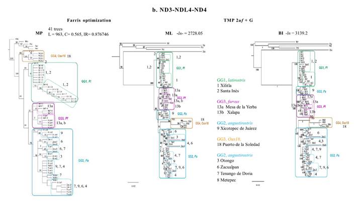
Figure 2 Topologies resulting from phylogenetic analyses using Maximum Parsimony (MP), Maximum Likelyhood (ML), and Bayesian Inference (BI) with sequences for the Cytochrome-b gene with 719 bases (a) and sequences for the NADH genes with 971 bases (b). The numbers on the nodes indicate percentage of support for the branches per 1000 bootstrap replicas. See text for description of support values. See Appendix for details.
In addition to the lack of genetic divergence between Xilitla (GL1) and Santa Inés (GL2) in GG1 (Pl) in the NADH genes, there were two additional exceptions (Table 2) for significant divergence between the GLs from the intermediate GGs (GG2 Pa; GG3 Pf). In the Cytb gene, Metepec, Hidalgo (GL8, GG2, Pa) showed the least genetic divergence from the type localities of either GG2 (GL6, Zacualpan, Veracruz) or GG3 (Pf, GL13, Xalapa, Veracruz), regardless of the geographic distance (24.4 and 174 km, respectively). Likewise, for the NADH genes, the lack of genetic divergence involved only GLs from GG2 (Pa), including Tenango de Doria (GL7), located almost 150 km from Tlanchinol (GL4) in Hidalgo, and 32 km distant from Xicotepec de Juárez (GL9) in Puebla (Table 2). All remaining GLs at each gene possessed significant distances of genetic divergence (Table 2), regardless of their geographic proximity (e. g., 20 km between Mesa de la Yerba and Xalapa, in Veracruz, NADH). These results suggest that there may be different genetic subgroups within the intermediate portion of the geographic range.
Table 2 Genetic divergence in mitochondrial genes Cytochrome-b (A) and ND3-ND4L-ND4 (B), depicted by distances of Tamura and Nei’s (N-T, below diagonal) between pairs of Group Localities (GL#) in the Genetic Groups (G1-4), arranged in a NW-SE direction. Geographic distances (e. g., straight lines for km between GLs) are also shown as reference (above diagonal). Number of asterisks depict significant N-T genetic distances among and within GLs (and GGs), according to level of p-values: * p < 0.05 and ** p < 0.01; bold distances had non-significant p-values (> 0.05). Colors correspond to color-code in Figures.
| A. Cytochrome-b | ||||||||||||
|---|---|---|---|---|---|---|---|---|---|---|---|---|
| GL# | GG | Code | Xili | Tlan | Zacu | TeDo | Metp | Huau | Xalp | PtSl | ||
| 1 | GG1 | Xili | 0 | 65.17 | 137.18 | 147.53 | 158.52 | 182.87 | 322.11 | 447.53 | ||
| 4 | GG2 | Tlan | 0.96* | 0 | 124.61 | 136.07 | 95.83 | 166.99 | 256.61 | 380.72 | ||
| 6 | GG2 | Zacu | 0.92* | 0.73* | 0 | 14.65 | 24.41 | 45.24 | 190.24 | 306.96 | ||
| 7 | GG2 | TeDo | 0.93* | 0.53** | 0.55* | 0 | 19.93 | 34.38 | 177.45 | 298.48 | ||
| 8 | GG2 | Metp | 0.91** | 0.69* | 0.28 | 0.48** | 0 | 27.99 | 173.64 | 292.28 | ||
| 10 | GG2 | Huau | 0.97* | 0.97** | 0.93** | 0.92** | 0.92* | 0 | 146.03 | 271.31 | ||
| 13 | GG3 | Xlpa | 0.89* | 0.86** | 0.73* | 0.82** | 0.65 | 0.90** | 0 | 161.77 | ||
| 18 | GG4 | PtSl | 0.97* | 0.98** | 0.96** | 0.96* | 0.96* | 0.98** | 0.96** | 0 | ||
| B. ND3-ND4l-ND4 | ||||||||||||
| GL# | GG | Code | Xili | SaIn | Oton | Tlan | Zacu | TeDo | XiJu | MsYb | Xlpa | PtSl |
| 1 | GG1 | Xili | 0 | 21.86 | 58.62 | 65.17 | 137.18 | 147.53 | 175.43 | 342.11 | 322.11 | 447.53 |
| 2 | GG1 | SaIn | 0.1 | 0 | 46.76 | 58.29 | 124.61 | 136.07 | 165.7 | 332.87 | 312.87 | 429.32 |
| 3 | GG2 | Oton | 0.81** | 0.71* | 0 | 17.51 | 78.83 | 82.88 | 118.76 | 286.55 | 266.55 | 386.75 |
| 4 | GG2 | Tlan | 0.80** | 0.75** | 0.36* | 0 | 137.18 | 147.53 | 117.07 | 276.61 | 256.61 | 380.72 |
| 6 | GG2 | Zacu | 0.75** | 0.66** | 0.20** | 0.16* | 0 | 14.65 | 46.46 | 210.24 | 190.24 | 306.96 |
| 7 | GG2 | TeDo | 0.83** | 0.80* | 0.39* | 0.04 | 0.22* | 0 | 32.10 | 197.45 | 177.45 | 298.48 |
| 9 | GG2 | XiJu | 0.75** | 0.66** | 0.43** | 0.28* | 0.3** | 0.29 | 0 | 167.10 | 147.10 | 276.65 |
| 13 | GG3 | MsYb | 0.84** | 0.83** | 0.68** | 0.65** | 0.53** | 0.76** | 0.44** | 0 | 20.00 | 161.67 |
| 13 | GG3 | Xlpa | 0.79** | 0.74** | 0.64* | 0.65** | 0.56** | 0.71** | 0.46** | 0.26** | 0 | 181.67 |
| 18 | GG4 | PtSl | 0.84** | 0.76** | 0.72** | 0.78** | 0.72** | 0.78* | 0.73** | 0.83** | 0.77** | 0 |
The genetic structure of the GLs in GG1-4 (Table 3) with the Cytb gene indicated that the two populations at the end of the geographic range (GL Xilitla, GG1 Pl; GL18 Puerto de la Soledad, GG4 Oax18) had the lowest genetic divergence. The northern populations of GG2 (Pa), Huauchinango in northern Puebla (GL10) and Tlanchinol in northern Hidalgo (GL4) were the most genetically conserved. Tenango de Doria, a southern location in Hidalgo (GL7) and to the southeast of the type locality of GG2 (Pa), Zacualpan, Veracruz (GL6), also was genetically conserved with a divergence slightly higher than GL1 and GL18. Zacualpan (GL6), which is geographically closer to populations at Tenango de Doria (GL7) and to the populations of Metepec (GL8), showed twice the amount of genetic variation than the former but 50 % less than the latter. Finally, Xalapa (GL13), in central Veracruz and the type locality for GG3 (Pf), showed four times more genetic divergence than Metepec (GL8) and ranked as the most variable GL for the Cytb gene. However, the number of indels in the Xalapan sequences (Table 3) were responsible for the higher genetic diversity. Excluding these indels, Xalapa had genetic diversity more similar to Tenango de Doria (GL7, GG2 Pa) for the Cytb data.
The three NADH genes showed a relative higher amount of genetic diversity among GG1-4 than did the Cytb gene (Table 3). The GLs with the lowest genetic divergence were Mesa de la Yerba (GL13b, GG3 Pf) in central Veracruz and the most northern and distant Xilitla (GL1, GG1 Pl). Tenango de Doria (GL7 Pa) and Santa Inés (GL1 Pl) were the next least divergent localities. Xalapa (GL13 Pf) and Tlanchinol (GL4 Pa) possessed intermediate levels of genetic diversity with Tlanchinol (GL4 Pa) being similar to the northernmost populations in Puebla, Xicotepec de Juárez (GL9 Pa). Finally, although Puerto de la Soledad in northern Oaxaca was located geographically near Zacualpan (GL6 Pa) and Tenango de Doria (GL7 Pa), it was genetically divergent based on the NADH genes.
Haplotype networks in the Internal Group. As in all phylogenetic topologies with molecular data (Figures 2, 4), each GG1-4 is readily recognizable in the haplotype networks (Figure 3) because all haplotypes from the GLs joined, regardless of geographic proximity between their respective GLs (Figure 1b, Table 2). Both haplotype networks reflected the overall geographical distribution of the G1-4 (Figures 1, 3), with sequences of GG1 (latirostris, Pl) and GG4 (Oax18) at the geographical extremes, and GG2 (angustirostris, Pa) and GG3 (furvus, Pf) join in the intermediate zone. However, in both haplotype networks, GG3 (Pf) appears to be closer to GG1 (Pl) than GG2 (Pa). The distinctiveness of GG1-4 is supported by the large amount of the variance as seen in the AMOVA (78.30 % in Cytb and 63.24 % in the NADH genes, Table 1). The haplotype networks are consistent in depicting geographic representation (Table 4, Figure 1, Appendix), but differ in the intrinsic amount of genetic variation when Cytb is compared to NADH (Tables 1, 2). Accordingly, each network displayed its own number of mutations (steps in each branch), including those between known haplotypes, between haplotypes and unknown haplotypes, and between unknown haplotypes. Unknown haplotypes appear as “UnkH” in Table 4 and as red diamonds on Figure 3.
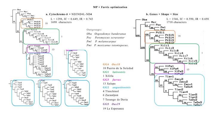
Figure 3 Haplotype networks for the Genetic Groups within the Ingroup in the Cytochrome-b gene (a) and in the NADH genes (b). Red diamonds depict unknown haplotypes; digits in the joining lines among haplotypes, indicate the number of mutations (genetic divergence); the underlined haplotype H4 is shared in two nearby group localities in Hidalgo. The tones of the colors aim to facilitate location of the group localities within the same GG. See text and Table 4.
Table 3 Indexes of genetic diversity (Pi) in the representative populations of the genetic groups (GG1-4) of the Ingroup, indicating the related statistics (Theta Pi with one standard deviation, SD), the number (No.) of mutations by type, and the respective mean with its standard deviation (SD) for cytochrome-b and ND3-ND4L-ND4. Colors correspond to those in the Figures. See Appendix for details.
| Cytochrome-b | ||||||||||||
|---|---|---|---|---|---|---|---|---|---|---|---|---|
| Group Locality# | GL1 | GL4 | GL6 | GL7 | GLG8 | GL10 | GL13 | GL18 | ||||
| Genetic Group | GG1 | GG2 | GG2 | GG2 | GG2 | GG2 | GG3 | GG4 | ||||
| GL Code | Xili | Tlan | Zacu | TeD | Metp | Huau | Xlpa | PtSl | Mean | SD | ||
| n of sequences | 8 | 7 | 3 | 8o | 2 | 9 | 4 | 12 | ||||
| Statistic | Genetic diversity | |||||||||||
| Pi | 1.43 | 0.86 | 5.33 | 3 | 10 | 0.22 | 61.5 | 1.44 | 10.47 | 19.5 | ||
| Theta Pi | 1.43 | 0.86 | 5.33 | 3 | 10 | 0.22 | 61.5 | 1.44 | 10.47 | 19.5 | ||
| SD Theta Pi | 1.1 | 0.78 | 4.4 | 1.99 | 10.49 | 0.33 | 40.56 | 1.06 | 7.59 | 12.8 | ||
| Mutations, number of | ||||||||||||
| transitions, ts | 5 | 2 | 7 | 11 | 10 | 0 | 8 | 6 | 6.13 | 3.5 | ||
| transversions, tv | 0 | 0 | 1 | 1 | 0 | 1 | 1 | 1 | 0.63 | 0.5 | ||
| substitutions, sb | 5 | 2 | 8 | 12 | 10 | 1 | 9 | 7 | 6.75 | 3.6 | ||
| indels, in | 0 | 0 | 0 | 0 | 0 | 0 | 114 | 0 | 14.25 | 37.7 | ||
| Sum | 10 | 4 | 16 | 24 | 20 | 2 | 132 | 14 | ||||
| No. of ts sites | 5 | 2 | 7 | 11 | 10 | 0 | 8 | 6 | 6.13 | 3.52 | ||
| No. of tv sites | 5 | 2 | 7 | 11 | 10 | 0 | 8 | 6 | 0.63 | 0.48 | ||
| No. of ss sites | 5 | 2 | 8 | 12 | 10 | 1 | 9 | 7 | 6.75 | 3.6 | ||
| No. of in sites | 0 | 0 | 0 | 0 | 0 | 0 | 114 | 0 | 14.25 | 37.7 | ||
| Sum | 15 | 6 | 22 | 34 | 30 | 1 | 139 | 19 | ||||
| ND3-ND4L-ND4 | ||||||||||||
| Group Locality# | GL1 | GL2 | GL3 | GL4 | GL6 | GL7 | GL9 | GL13 | GL13 | GL18 | ||
| Genetic Group | GG1 | GG1 | GG2 | GG2 | GG2 | GG2 | GG2 | GG3 | GG3 | GG4 | ||
| Code | Xili | SaIn | Oton | Tlan | Zacu | TeDo | XiJu | MsY | Xlpa | PtSl | Mean | SD |
| n of sequences | 13 | 5 | 3 | 7 | 7 | 4 | 7 | 6 | 5 | 12 | ||
| Statistic | Genetic diversity | |||||||||||
| Pi | 7.9 | 9.83 | 28.7 | 13.05 | 23.29 | 9 | 18.19 | 6.33 | 12 | 22.8 | 15.11 | 7.26 |
| Theta Pi | 7.9 | 9.83 | 28.7 | 13.05 | 23.29 | 9 | 18.19 | 6.33 | 12 | 22.8 | 15.11 | 7.26 |
| DE Theta Pi | 4.42 | 6.83 | 21.8 | 7.68 | 13.4 | 6.28 | 10.55 | 4.04 | 7.67 | 14.21 | 9.69 | 5.19 |
| Mutations, number of: | ||||||||||||
| transitions, ts | 9 | 11 | 30 | 27 | 39 | 11 | 28 | 10 | 25 | 34 | 22.4 | 10.6 |
| transversions, tv | 18 | 8 | 13 | 11 | 27 | 6 | 8 | 5 | 4 | 19 | 11.9 | 7.02 |
| substitutions, sb | 27 | 19 | 43 | 38 | 66 | 17 | 36 | 15 | 29 | 53 | 34.3 | 15.6 |
| indels, in | 1 | 0 | 0 | 0 | 0 | 0 | 0 | 0 | 0 | 0 | 0.1 | 0.3 |
| Sum | 30 | 38 | 86 | 76 | 132 | 34 | 70 | 30 | 58 | 106 | ||
| No. of ts sites | 9 | 11 | 30 | 27 | 39 | 11 | 28 | 10 | 25 | 34 | 22.4 | 10.6 |
| No. of tv sites | 9 | 11 | 30 | 27 | 39 | 11 | 28 | 10 | 25 | 34 | 11.9 | 7.02 |
| No. of ss sites | 27 | 19 | 43 | 38 | 64 | 17 | 36 | 15 | 29 | 53 | 34.1 | 15.2 |
| No. of in sites | 1 | 0 | 0 | 0 | 0 | 0 | 0 | 0 | 0 | 0 | 0.1 | 0.3 |
| Sum | 46 | 41 | 103 | 92 | 142 | 39 | 92 | 35 | 79 | 121 |
The 53 sequences in the Cytb gene coalesced into 24 distinctive haplotypes inside the eight GLs representing GG1-4 with one exception (Table 4, Figure 3a). GG2 (Pa) from Hidalgo, Tenango de Doria (GL7), and Metepec (GL8), shared the same haplotype (H4). For Cytb, all GLs had 1-2 shared haplotypes except for Metepec (GL8). The number of mutations ranged from 1 to 29 with most found within the GGs, except for each of the type localities of GG3 (Pf, GL13, H21, 6) and GG3 (Pa, GL6, H22, 4). Among GGs represented by a single GL (Figure 3a), populations from Oaxaca (GG4 Oax18) had no unknown haplotypes, whereas San Luis Potosí (GG1 Pl) and (GG3 Pf) had one each. GG2 (Pa) had five GLs and included seven unknown haplotypes (Figure 3a), most of which joined the GLs from Hidalgo (GL4, GL7, and GL8) with Zacualpan, Veracruz (GL6), the type locality of angustirostris. GL4 (Tlanchinol) and GL7 (Tenango de Doria), located 82.93 km apart (Table 2), joined through two mutations; whereas an unknown shared haplotype joined four geographically closer GLs (Table 2) through either 1, 2, or 4 mutations. Zacualpan (GL6) joined through to Metepec (GL8, 21.41 Km) or Tenango de Doria (14.65 km) by a single mutation (H4). Tenango de Doria (GL7) and Metepec (GL8), which are separated by 19.93 km, also differed by one mutation. The most divergent subpopulation in GG2 (Pa) was Huauchinango, Puebla (GL10) which is 28 km from Metepec (GL8) but that was separated from it (and from all the other GLs) by 5 to 6 unknown haplotypes and at least 11 mutations.
Although Huauchinango (GL10) is the most proximate (271.31 km) subpopulation of GG2 (Pa) to Puerto de la Soledad, Oaxaca (GG4 Oax18), the number of mutations between these two GGs scored highest in the Cytb network, with 29 mutations and 1 to 2 unknown haplotypes (Figure 3a). Branches joining GG2 (Pa) to GG3 (Pf) included 3 to 7 unknown haplotypes. In the network analysis (Figure 3a), Xalapa (GL13, Pf) was genetically divergent from Tlanchinol (GL4, 256.6 km) and to the group formed by Zacualpan (GL6, 190. 24 km), Tenango de Doria (GL7, 177.45 km), and Metepec (GL8, 173.64) by 10 mutations. Xalapa (GL13 Pf) compared to that of Huauchinango (GL10), to which it is geographically closer (146.04 km), differed by 11 mutations. Finally, the branches between GG1 (Pl, Xilitla, San Luis Potosí, GL1) and GG3 (Pa, Xalapa, Veracruz, GL13) showed a genetic divergence of 19 mutations (Figure 3a).
Table 4 Haplotypes (H#) analyzed in gene networks for Cytochrome-b and three NADH genes, according to OTU (genetic group, GG1-4, taxonomic entity and key). Geographic data include the group localities (GL#) in a NW-SE direction (see Figure 1b); the asterisk (*) indicates type localities or first known localities. The total number of genetic sequences (#Sequences) in each OTU appears in the next column with the GL code, whereas in the last column, the number inside parenthesis indicates how many were shared in a common haplotype. See Appendix 1. Colors for OTUs are as in Figure 3.
| OTU | GL#. Name, State | GL Code | Haplotypes | Common H#s |
|---|---|---|---|---|
| # Sequences | H# | (#Sequences) | ||
| Cytochrome -b gene | ||||
| GG1 latirostris Pa | 1. Xilitla, San Luís Potosí* | Xili 1-8 | H15-H18 | H15(5) |
| GG2 angustirostris Pa | 4. Tlanchinol, Hidalgo | Tlan 1-7 | H12-H14 | H13 (3), H14(2) |
| 6. Zacualpan, Veracruz* | Zacu 1-3 | H22, H23 | H22(2) | |
| 7. Tenango de Doria, Hidalgo | TeDo 1-9 | H4, H10-H11 | H10(7), H4(Metpc) | |
| 8. Metepec, Hidalgo | Metp 1-2 | H3, H4 | H4(TeDo) | |
| 10. Huauchinango, Puebla | Huau 1-9 | H1-H2 | H1(8) | |
| GG3 furvus Pf | 13. Xalapa, Veracruz* | Xlpa 1-4 | H19-H21, H20 | H20(2) |
| GG4 unknown Oax18 | 18. Puerto de la Soledad, Oaxaca* | PtSl 1-12 | H5-H9 | H5(8) |
| ND3-ND4L-ND4 genes | ||||
| GG1 latirostris Pa | 1. Xilitla San Luís Potosí* | Xili 1-13 | H1-H10 | H3(3) ,H1(2) |
| 2. Santa Inés, Qro (SaIn1-4) | SaIn 1-4 | H11-H14 | none | |
| GG2 angustirostris Pa | 3. Otongo, Hgo (Oton1-4) | Oton 1-4 | H22-H24 | none |
| 4. Tlanchinol, Hidalgo | Tlan 1-4 | H15-H21 | none | |
| 6. Zacualpan, Veracruz* | Zacu 1-7 | H25-H31 | none | |
| 7. Tenango de Doria, Hidalgo | TeDo 1-4 | H32-H35 | none | |
| 9. Xicotepec de Juárez, Pue (XiJu1-7) | XiJu 1-7 | H36-H42 | none | |
| GG3 furvus Pf | 13a. Xalapa, Veracruz* | MsYb 1-6 | H43-H48 | H50(2) |
| 13b. Mesa de la Yerba, Veracruz* | Xlpa 1-6 | H49-H52 | none | |
| GG4 unknown Oax18 | 18. Puerto de la Soledad, Oaxaca* | PtSl 1-5 | H53-H57 | none |
In the NADH genes network (Figure 3b), the 58 sequences resulted in 57 distinctive haplotypes, the sole exception being H50 from Mesa de la Yerba in central Veracruz (GL13, GG3 Pf), which was presented by two sequences. With the exception of Puerto de la Soledad, Oaxaca (GL18, GG4 Oax18), all other GGs had more than one GLs representing them: two in either GG1 (Pl) and GG3 (Pf) and five in GG2 (Pa). Overall, the number of mutations in the network branches ranged from 1 to 31. In the NADH network, the total number of unknown haplotypes was slightly more than triple that found in Cytb (Figure 3b). Although most haplotypes from the same GL were spatially closer, there was more intermingling among haplotypes from different GLs, thus allocating haplotypes among some GLs. Furthermore, the higher and more fluctuating number of mutations among the GLs, the greater intermingling of haplotypes from different GLs in the same genetic group. The lower number of shared haplotypes rendered a lower percentage of variance explained by the variation among GG1-4 in the AMOVA (Table 1). For the NADH genes, variation within subpopulations (GLs) accounted for a higher amount of variance than in the Cytb gene.
In GG4 (Oax18, GL1), no sequence joined another except through unknown haplotypes (number of mutations was 4, 11, 15, and 23; Figure 3b). H53, the most divergent haplotype, diverged by 31 mutations from an unknown haplotype that join a GL of GG2 (Pa) from Puebla (GL9, Xicotepec de Juárez, 276 km) and two from Hidalgo (GL7, Tenango de Doria, 298 km; GL4 Tlanchinol, 380 km). The haplotypes of three GLs formed their own subpopulation and shared haplotypes from others through unknown haplotypes. These three GLs contained 1 to 6 mutations and only Tenango de Doria (GL7; H34, H35) and Xicotepec de Juárez (GL9; H38, H20) had haplotypes that joined to the same subpopulation. Xicotepec de Juárez, Puebla (GL9) is 32 km from Tenango de Doria (GL7) and 117 km from Tlanchinol (GL4) and their haplotypes diverge from unknown haplotypes by 1, 2, or 6 mutations. Only H15 from Tlanchinol (GL4) joins Otongo (GL3), 17 km distant, through a genetic divergence of at least 17 unknown haplotypes. The level of divergence in the sequences from Otongo (GL3) includes 1, 7, and 30 mutations from unknown haplotypes. The sequences from the type locality Zacualpan, Veracruz (GL6) also formed a separate group but joined by 7 or 11 mutations to Otongo (GL3), 78 km away. Most genetic divergence among subpopulations contained 1 or 3 mutations, however, haplotypes had 6, 8, 12, and 31 mutations to an unknown haplotype. Therefore, the overall number of mutations in GG2 (Pa) was high. Consistent with its intermingling pattern, GG2 (Pa) joins to GG3 (Pf) through clusters of two different subpopulations separated by 46 km (Zacualpan GL6, Xicotepec de Juárez GL9). The route from Zacualpan (GL6 Pa) involved 14 to 17 mutations between haplotypes connecting it to Xalapa (GL13 Pf). The alternative route from Xicotepec de Juárez (GL9 Pa) to Xalapa (GL13 Pa) encompasses 13 mutations between unknown haplotypes (GL9 is 147 km from GL13).
The two GLs in GG3 (Pf) are 20 km distant and joined by either 5 or 15 mutations (Table 2). In Xalapa (GL13a), the number of mutations from an unknown haplotype ranged from 1 to 3, and 6, but in Mesa de la Yerba (GL13b) they were higher with 1, 4, 9, or 12 mutations. The only joining of two haplotypes from the same subpopulation (Figure 3b) occurred in Mesa de la Yerba, which had a single mutation between haplotype H50 and H51. H50 was the only shared haplotype in the entire NDH network. Between GG3 (Pf) and GG1 (Pl), there are 23 mutations segregating the two unknown haplotypes to which 5 or 10 mutations join Mesa de la Yerba (GL13a) and another one joined Xilitla, San Luis Potosí (GL1). These two GLs are 322 km distant. In Xilitla (GL1), the number of mutations from a haplotype to an unknown haplotype was 1, but there also were 2, 5, 7, and 10 mutations. The number of mutations between GL1 and Santa Inés, Querétaro (GL2), was 2 or 4, and the latter joined to unknown haplotypes by 1, 2, or 10 mutations.
Combined datasets. In the MP analyses for combined datasets (Figure 4), all OGs were distinct from the members of the IG and each GG1-4 was readily recognizable with support values of > 90 to 100 %. Oba was always at the root, whereas the sister group to all IG was (Mcr(Poc(Pml Pmt))). In this sister group, only the clade of Pml and Pmt was well supported (85%, 86%). In the IG, the sequences from Puerto de la Soledad, Oaxaca (GG4, Oax18) were located basally and separated from other GGs. In the most derived clade, sequences from Xilitla, San Luis Potosí (GG1 Pl) showed full support and separated from a sister subclade with sequences from the two remaining GGs. Clade support was high in ML but lowered in the IB topology for the sequences from Xalapa, Veracruz (GG3 Pf) and in GG2 (Pa) with all the remaining sequences from Hidalgo and Veracruz (GG2 Pa). However, the clades of these two GGs were distinctive from each other and with strong support.
The MP strict consensus cladogram combining all molecular sequences (Figure 4a) resulted from four most parsimonious trees (L = 1298, IC = 0.649, IR = 0.743). The differences among these original trees (Figure 4a) were due to the relative position of the specimens of GG2 (Pa) from the two group localities in Hidalgo, Tlanchinol (GL4) and Tenango de Doria (GL7) with respect to the specimens from Zacualpan, Veracruz (GL6). The addition of morphometric data in the multicharacter phylogeny (Fig 4b) resolved the aforementioned discrepancies in a single, though longer tree (L = 1546, IC = 0.590, IR = 0.698). In agreement to its geographic location, a sequence from Tlanchinol (GL4) preceded a group with all the sequences from Zacualpan (GL6) and one sequence from Tenango de Doria (GL7). This sister clade included sequences from GL4 and GL7 that are geographically more distant (Table 2) and poorly supported (8 %). However, some clades ranked from moderate (Tlanchinol, 50 %) to acceptable (Zacualpan and Tenago de Doria, or the latter alone, with 76 % each). In both combined datasets with genetic data (Figure 4), branches defining subclades associated with the separation of every GG were fully (100 %) or very highly supported (90 to 99 %).

Figure 4 Topologies from selected populations of Peromyscus furvus, integrating two types of mitochondrial genes in a strict consensus cladogram (a; note the four outcomes for GG2), and the former with 28 morphometric characters for skull shape and size in a completely resolved single phylogenetic tree (b). The numbers on the nodes indicate percentage of support for the branches per 1000 bootstrap replicas. See text for description of support values.
Percentage genetic distances within the IG and with all OTUs for the Cytb gene. In the analysis of the IG (Table 5a), the larger genetic distances occurred between GG4 (Oax18) from Puerto de la Soledad, Oaxaca (GL18) and the other GGs (6.6 to 7.8 %), with the exception of Metepec, Hidalgo (GL8) of GG2 (angustirostris) which was <2 %. Likewise, although of smaller magnitude, the genetic distances associated with GG1 (latirostris) from Xilitla, San Luis Potosí (GL1) showed segregation from all the other GGs (3.8 to 7.8 %). GG3 (furvus) from Xalapa, Veracruz (GL13) differentiated from GG1 (latirostris, 3.8 %) and especially from GG4 (Oax18, 7.6 %). However, the genetic distances of GG3 (furvus) were lower (2.4 to 3.0 %) with respect to the remaining localities in Hidalgo, Puebla, and Veracruz (corresponding to GG2, angustirostris). The variation among the localities within GG2 (angustirostris) ranged 0.7 to 2.7 %. Noticeably, these analyses also showed minimal genetic distances even among individuals from the same locality (Table 5a) both in Metepec, Hidalgo (GG2 angustirostris) and in Xalapa, Veracruz (GG3 furvus).
In the genetic distances including all OTUs (Table 5b), all comparisons among the OGs and IGs, averaged >11 % with an average genetic divergence among the ten OTUs of 16.2 % (range values, 11.8 to 22.9 %); among the OGs from the IG, the values were 15.6 % (11.8 to 19.8 %). Peromyscus ochraventer (Poc, 18.4 %) had the greatest divergence from the IG, followed by O. banderanus (Oba, 16.4 %) and P. melanocarpus (Pml, 16.1 %). P. mexicanus totontepecus (Pmt, 14.2 %) and M. cryophilus (Mcr, 13.0 %) showed the lower genetic distances from the IG. The overall average genetic divergence of the IG from all the OGs was 15.6 %. GG3 (Pf, 16 %) was the most divergent to all OGs, followed by both GG2 (Pa, 15.7 %) and GG4 (Oax18, 15.7 %), whereas GG1 (Pl, 15.1 %) was slightly less divergent. When pooled together, GG3 (Pl) and GG2 (Pa) were slightly more divergent from the OGs (15.9 %) than GG4 (Oax18). When the IG was individually compared with all three Peromyscus in the OG (Poc, Pml, and Pmt), they diverged by an average genetic distance of 16.1 % if the GG3 (furvus) and GG2 (angustirostris) were pooled together, but with an average distance of 14.2 % if they were separated.
GG1-4 differed from each other with lower average genetic distances (5.9 %, 2.8 to 8.4 %; Table 5b). Puerto de la Soledad (GG4 Oax18) had an average genetic distance of 7.9 % from GG1-3. GG1 (latirostris) differed from GG2-4 by 5.8 %, and GG3 (furvus) and GG2 (angustirostris) diverged from the other three GGs by 5 %. Either pooled together or alone, the two latter GGs had an average divergence of 6.0 to 6.1 % from the two geographically extreme GG1 (latirostris) and GG4 (Oax18), but were 7.7 % from GG4 and 4.5 % from GG1. The least average genetic distance (2.8 %) was between GG2 (furvus) and GG3 (angustirostris).
Finally, the average genetic distance among the OGs was 17.5 % (12.5 to 22.9 %). P. ochraventer (Poc, 20.3 %) had the most divergent average genetic distance, followed by O. banderanus (Oba, 18.5 %). P. melanocarpus (Pml, 16.9 %) and P. mexicanus totontepecus (Pmt, 16.7 %) and M. cryophilus (Mcr, 15.1 %) showed lower genetic divergence. The least divergent OGs were Pml and Pmt (12.5 %), and the most divergent were Poc and Pml (22.9 %).
Table 5 Percentage genetic divergence (%) of the Tamura and Nei genetic distances, sensuBradley and Baker (2001), for the Cytochrome-b gene in the genetic groups (GG1-4) of the ingroup (a) and in all the species examined herein (b). Genetic distances between pairs of entities appear below the diagonal the numbers on diagonal in the genetic groups are distances within populations (GLs).
| a. Genetic Groups | GL#. Name, State | GL1 | GL4 | GL6 | GL7 | GL8 | GL10 | GL13 | GL18 |
|---|---|---|---|---|---|---|---|---|---|
| GG1 latirostris Pl | 1. Xilitla, San Luis Potosí | 0.0 | |||||||
| GG2 angustirostris Pa | 4. Tlanchinol, Hidalgo | 4.4 | 0.0 | ||||||
| 6. Zacualpan, Veracruz | 4.5 | 1.1 | 0.0 | ||||||
| 7. Tenango de Doria, Hidalgo | 5.0 | 0.7 | 1.2 | 0.0 | |||||
| 8. Metepec, Hidalgo | 4.1 | 1.2 | 0.7 | 1.2 | 0.01 | ||||
| 10. Huauchinango, Puebla | 4.9 | 2.4 | 2.5 | 2.7 | 2.6 | 0.0 | |||
| GG3 furvus Pf | 13. Xalapa, Veracruz | 3.8 | 2.4 | 2.8 | 3.0 | 2.7 | 2.5 | 0.01 | |
| GG4 unknown Oax18 | 18. Puerto de la Soledad | 7.8 | 7.2 | 7.3 | 6.7 | 1.2 | 6.6 | 7.6 | 0 |
| b. All OTUs | Oba | Mcr | Poc | Pml | Pmt | Pl | Pff | Pfa | Oax18 |
| Osgoodomys banderanus, Oba | |||||||||
| Megadontomys cryophilus, Mcr | 16.7 | ||||||||
| Peromyscus ochraventer, Poc | 20.3 | 15.9 | |||||||
| P. melanocarpus, Pml | 17.9 | 14.1 | 22.9 | ||||||
| P. mexicanus totontepecus, Pmt | 18.9 | 13.5 | 21.9 | 12.5 | |||||
| P. latirostris / P. f. latirostris, Pl | 15.8 | 13.7 | 16.9 | 15.0 | 14.0 | ||||
| P. f. furvus, Pff | 16.9 | 13.3 | 19.1 | 16.8 | 13.8 | 5.0 | |||
| P. f. angustirostris Pfa | 16.1 | 13.1 | 19.8 | 15.6 | 14.1 | 4.0 | 2.8 | ||
| Unknown Peromyscus from Oax18 | 16.8 | 11.8 | 17.8 | 17.1 | 14.9 | 8.4 | 7.3 | 8.1 |
Discussion
The results presented herein were obtained from several analyses, including single-character phylogenies and all methods combined (MP, ML, and BI). Regardless of method, GG1 (latirostris, Pl), GG3 (furvus, Pf), and GG4 (Oax18) were always distinct because their sequences were reciprocally monophyletic. All analyses of the Cytb gene and the MP analyses for the NADH genes yielded a topology nearly identical to that reported by Harris et al. (2000:2131-2). However, the probabilistic topologies of the NADH genes concurred with the findings of Ávila-Valle et al. (2012:171). In Harris et al. (2000), the most distinctive entity was GG4 (Oax18), followed by GG1 (Pl), whereas in Ávila-Valle et al. (2012) the latter was the most distinctive entity and GG4 (Oax18) was associated with GG2 (Pa). Although these authors pointed out the distinctiveness of these two GGs, they did not propose their formal recognition. It is clear that the populations in the intermediate zone of the distribution range posed a challenge to interpreting the phylogenetic relationships among them, especially because their subpopulations (GLs) were not monophyletic in several of their topologies (Harris et al. 2000; Ávila-Valle et al. 2012). Aside from Huauchinango, Puebla (GL10), Otongo, some sequences of Tlanchinol, Tenango de Doria from Hidalgo, and some sequences of Mesa de la Yerba and Xalapa from Veracruz, combinations of sequences from different GLs (i. e., Zacualpan-Metepec-Tenango de Doria) had greater support than did all sequences representative of GG2 (Pa) in topologies of single types of genes. Similar results were obtained from the variance components in the AMOVA and in the haplotype networks herein.
Differences in the outcomes of these topologies were based on the method (non-parametric MP, parametric ML, BI; e. g., Steel and Penny 2000; Sober 2004), especially in the methods used to calculate branch length; probably due to different ontological and epistemological assumptions (De Luna 1995). Another possible source for disconcordance among topologies could have been from the evolutionary model used in the probabilistic methods and its relationship with the evolutionary assumptions in the MP analysis. The GTR I + G (GTR) used in the Cytb is more realistic, though more complex and thus with more probability of error because it considers six substitution parameters; whereas, the more simple model TMP 2 uf + G (TMP2) only has three parameters (Posada 2008). The GTR model, by assigning the same importance to the changes from one base to another and vice versa, is more like the Farris optimization model in MP analysis (Farris 1970; Lipscomb 1998). However, GTR considers different probabilities for the different types of mutations (Tavare 1986) and assigns a specific value to particular types of mutations. Conversely, the TPM2 model accepts and evaluates only three forms of base substitutions (Kimura 1981), thus ignoring possible informative mutations for phylogenetic analyses, unlike the Farris (1970) optimization. Use of GTR as an evolutionary model for the Cytb, with or without invariant sites, is quite frequent in studies on the systematics of Peromyscus (e. g., Harris et al. 2000; Bradley et al. 2007; Bradley et al. 2014; Platt et al. 2015; and other references therein and herein). However, exploration of TPM2 in Peromyscus (Walker and Greenbaum 2006; Ávila-Valle et al. 2012; Castañeda-Rico et al. 2014) and other species (León-Paniagua et al. 2007) is just beginning.
Ávila-Valle et al. (2012) also used the GTR model and obtained the same topology as presented herein for the NADH genes, even when they examined only whole ND3-ND4 sequences (1,043 base pairs). Therefore, the differences between the topologies may be due to a different evolutionary rate for nucleotide substitution (synonymous and non-synonymous) between the mitochondrial genes. Cytb evolves faster than do any of ND3, ND4L and ND4 genes in other mammalian orders (primates, carnivores, perissodactyls, and cetaceans; Pesole et al. 1999) and may have caused the disconcordance among topologies. For non-synonymous mutations, the rate of change for Cytb is at least two times faster than in any of the NDAH genes. For synonymous mutations, the rate of change in ND3 is 50 % less than that of the ND4 and Cytb, and the rate of change in ND4L is 25 % less than the Cytb and NADH genes. Therefore, GG4 may have grouped with GG2 and GG3 because of the influence of the ND3 and ND4L genes, whereas sequences from Cytb clearly separated it from the other GGs. The rate of change in Cytb has proven to be adequate to discern both intraspecific (intrapopulation, intrasubspecific, intraspecific) and intrageneric (sister species, interspecific) variation sensuBradley and Baker (2001). It also is likely that our adjustment in the number of bases in the GI (Pl) and the OG in the ND3-ND4L-ND4 genes allowed us to avoid possible inconsistencies between the sequences recovered from the literature and GenBank due to indels.
In our integrated phylogeny, based on all characters, we used the same epistemological approach to perform our analyses under the same evolutionary model (Farris optimization) and method (MP) in the TNT package (Goloboff et al. 2006). The decision to overcome technical restrictions for analyzing a big character matrix with different type characters allowed us to test the behavior of NADH genes under a more open evolutionary scenario. Moreover, it allowed us to include continuous morphometric characters for the shape and size of skull (Goloboff et al. 2006; Ramírez-Sánchez et al. 2016). As with the molecular data, we conducted single-character phylogenies for each size (linear measurements) and shape characters (morphogeometric configurations) with a much larger amount of individuals (in prep.), especially for size (i. e., those used in Ávila-Valle et al. 2012). Herein, morphometric characters solved the discrepancies among GLs in GG2 (Pa, Figure 2) in spite of reluctance of including them within combined molecular and morphometric phylogenies (Scotland et al. 2003). In other studies (e. g.,Lee and Camens 2009; Ledevin and Millien 2013), incorporation of morphometric characters into integrated phylogenies with molecular data has proven to be useful to understand and solve conflicting molecular outcomes.
After reduction of the number of genetic sequences in order to include only the GLs with both sequences, followed by an even more reduced number of GLs with all genetic and morphometric characters, GG1-4 appeared as well recognizable geographic and evolutionary entities with better supporting values compared to single-characters topologies. Herein, specimens from Puerto de la Soledad (GG4, Oax18), in the farther southern range, show the greatest genetic distances from the other GGs, and its geographic remoteness. Likewise, specimens (GG1, latirostris) from Xilitla, San Luis Potosí, with the second greatest geographic distances, showed twice the genetic divergence from specimens in the intermediate range. Finally, sequences from Xalapa, Veracruz and its surrounding locations (GG3, furvus), as well as those from Tlanchinol and Tenango de Doria, Hidalgo, and Zacualpan, Veracruz (GG2, angustirostris), were distinctly separated from each other as the subunits of a third genetic clade. Therefore, the monotypic status currently assigned to the populations in the overall distribution of P. furvus (Rogers and Skoy 2011) does not coincide with our genetic nor the morphometric data. Rather, the data presented herein confirms the morphometric (Musser 1964; Hall 1968; Martínez-Coronel et al. 1997; Ávila-Valle et al. 2012) and biochemical (Harris and Rogers 1999; Harris et al. 2000; Ávila-Valle et al. 2012) discrepancies reported previously.
Systematic and taxonomic remarks. Application of the genetic species concept (Wiley and Mayden 2000) sensuBaker and Bradley (2006), allows us to suggest the taxonomic level (clades and haplotypes clearly forming monophyletic groups) and the subspecific level (clades and shared haplotypes) of the distinctive genetic entities in the Cytb dataset. All GG1-4, with GG2-3 either separated (mean 14.2 %, 13.8 to 14.9 %) or pooled (16.1 %, 15.3 to 16.6 %), were similar in levels of genetic divergence as other congeneric species in the OG. When M. cryophilus and O. banderanus are included, the divergence level increased (15.6 %, 15.1 to 16 %) for the two genes. These levels of genetic distances among G1-4 indicate evidence supporting the recognition of genetic entities sensu Bradley and Baker (2001). The population of Puerto de la Soledad, Oaxaca (GG4) possessed the greatest genetic diversity of the four populations (GG1-4). GG4 had an average genetic distance of 7.5 % (or of 7.9 %, when the 10 OTUs were included), which is sufficient to distinguish it as a distinctive species from the other populations (GG1, latirostris; GG2, angustirostris, and GG3, furvus) sensu Bradley and Baker (2001) and Baker and Bradley (2006).
The northern population, (GG1, latirostris), possessed an average genetic distance of 4.2 % among GG1-3 (and of 4.9 % when the OGs are included in the analysis). Baker and Bradley (2006) mention a K2P distance interval of 2.8 to 10.8 % to validate species within Peromyscus, with several authors using a lesser distance than 7.0 %, although it is necessary to support genetic distance values with other kinds of evidence (Bradley and Baker 2001; Bradley et al. 2014). In the boylii species group, in addition to the genetic data of Cytb, the fundamental number of chromosomes and/or morphometric data have been used to describe new species in which the average lower limit of (i. e., the percentage genetic distance to its closest relative) is 4.3 % ± 1.1 SD (3.3 to 5.6 %). Following this logic, P. schmidlyi was described with a mean distance of 3.3 % from P. levipes (Bradley et al. 2004a), P. carletoni from P. levipes (3.4 %, Bradley et al. 2014), and P. kilpatricki from P. levipes (5.2 %, Bradley et al. 2016). Similarly, in the mexicanus species group, Lorenzo et al. (2016) described P. gardneri based on a K2P distance of 3.6 to 4.2 % from other species and reinforced the decision with morphometric data. In our analysis of linear (size) and morphogeometric (shape) characters, GG1 (latirostris) behaved as a separate entity, similar to that found in the morphometric data of Bradley et al. (2004a) and Lorenzo et al. (2016). In addition, GG1 (latirostris) has a larger skull size compared to GG2-4 (Martínez-Coronel et al. 1997; Ávila-Valle et al. 2012) and some distinctive qualitative cranial traits have been reported (Hall and Alvarez 1961; Musser 1964: Hall 1968).
GG2 (angustirostris) and GG3 (furvus) also possessed N-T genetic distances that averaged greater or similar to those K2P values reported for Peromyscus (Tiemann-Boege et al. 2000; Durish et al. 2004; Ordóñez-Garza et al. 2010). The average genetic distance between GG3 and GG2 was 2.7 % and 2.8 %, compared to other OTUs. Based on the logic presented in Bradley and Baker (2001), our results revealed that GG3 (furvus from the type locality Xalapa, Veracruz and its surroundings) and GG2 (angustirostris from Hidalgo, Puebla and locations further NW in Veracruz) would appear to be subspecies. The genetic distances between GG2 and GG3 are similar to that reported by Bradley et al. (2015) for two subspecies (ranging from 1.77 % in P. p. laceianus to 2.21 % in P. p. pectoralis). Similarly, Lorenzo et al. (2016) use a K2P genetic distance of 2.08-3.65% to define two subspecies of P. zarhynchus in Chiapas (P. z. zarhynchus and P. z. cristobalensis). Although our analyses were based on N-T distances, our overall conclusion concurs with the framework of Bradley and Baker (2001).
Finally, we suggest the possibility of additional subspecies within P. furvus. For example, ambiguities in the phylogenetic topologies were found by Harris et al. (2000) and Avila-Valle et al. (2012), as well as in haplotype networks presented herein. This is especially true for populations assigned herein to P. f. angustirostris to the north of Puebla (Huauchinango) and to the SE of the type locality (Zacualpan, Veracruz) in Hidalgo (i. e., Tlanchinol, Metepec, and Tenango de Doria). Sequences from the intermediate group localities are needed to resolve this issue. Further, sequences are needed from geographic areas such as Molango, Hidalgo, and from vegetational transition zones between Puebla and Veracruz (e. g., Rogers and Skoy 2011; Peralta-Moctezuma 2011).
Remarks for the furvus species group. Peromyscus furvus as currently conceived (sensu lato), contains multiple species and subspecies. The population of Puerto de la Soledad Oaxaca (GG4, Oax18) is a species nova, distinctive from P. furvus by its evolutionary divergence. This interpretation agrees with the genetic distances reported by Harris and Rogers (1999) for the allozyme PGDH, as well as with the possible biogeographic scenario proposed by Harris et al. (2000). Peromyscus latirostris from Xilitla, San Luis Potosí, and Santa Inés, Querétaro, is either a sister species to P. furvus, as suggested initially by Dalquest (1950), or is valid subspecies, P. f. latirostris. Our morphometric analyses (in prep.) strongly support the recognition of a separate species. Finally, populations along the intermediate zone (Hidalgo, Puebla, and Veracruz) represent at least two different subspecies, P. furvus angustirostris (as described by Hall and Álvarez 1961) and P. f. furvus (as described by J. A. Allen and Chapman 1897). Based on these findings, the furvus species group now comprises three species (P. latistrostis, P. species nova, and P. furvus) and at least two subspecies (P. f. angustirostris and P. f. furvus).
The pairing of P. m. totontepecus and P. melanocarpus agrees with the observation by Bradley et al. (2007) that P. melanocarpus did not seem to belong to the furvus species group, as it was more closely associated with species of the mexicanus species group (see Hooper 1968, Huckaby 1980). Peromyscus ochraventer, which also was considered a member of the furvus species group (Carleton 1989), behaved as an even more distant taxon from the furvus species group, as defined here and by others such as Wade et al. (1999) and Musser and Carleton (2005). Herein, P. ochraventer was more basal in all phylogenetic analyses, suggesting that this species is closer to the more derived difficilis species group (Durish et al. 2004; Bradley et al. 2007). The grouping of M. cryophilus with P. ochraventer in the OG is consistent with recent Cytb gene phylogenies, where this species and M. thomasi were genetically closer to P. furvus and the Oaxacan species nova (Bradley et al. 2007:1115) and to other subgenera such as Podomys and Neotomodon (Platt et al. 2015:712). Finally, except for the single molecular phylogenies with probabilistic methods in the NADH genes, O. banderanus was always basal and remained segregated from the other taxa. Its position at the base of the topology suggests an affiliation to the subgenus Haplomylomys, the basal most subgenus of Peromyscus in recent phylogenies of the genus (Bradley et al. 2004b, 2007; Platt et al. 2015).

