


 text new page (beta)
 English (pdf)
 Article in xml format
 Article references
 Send this article by e-mail
 Cited by SciELO
  Similars in
SciELO
Similars in
SciELO 
 Permalink
Introduction
Physical barriers and climatic variation within the distributional range of species are factors that influence the speciation process, and fluvial barriers have been considered to limit the dispersal of mammal species. This has been observed in many cryptic species inhabiting both sides of the Chihuahuan Desert and the drainage basins of the Altiplano Central (Mexico’s central highlands), including the rodent genera Chaetodipus, Geomys, Neotoma, and Peromyscus (Patton 1969; Walpole et al. 1997; Riddle et al. 2000a, 2000b; Edwards et al. 2001; Riddle and Hafner 2006; Patton et al. 2007; Neiswenter and Riddle 2010; Cornejo-Latorre et al. 2017; Neiswenter et al. 2019; Camargo and Álvarez-Castañeda 2020). In addition, this river seems to be a factor in the divergence between Perognathus flavus phylogroups within the Chihuahuan Desert, related to the expansion grasslands in the late Miocene and the Basin and Range geomorphology of the Miocene-Pliocene (Neiswenter and Riddle 2010).
The Chihuahuan Desert consists of portions divided by the Río Bravo (or Río Grande) and Río Conchos rivers (Figure 1). In addition, these rivers act as physical barriers in a climatic transition zone; the north encompasses the temperate Chihuahuan Desert, covered primarily by grasslands and Larrea, and the south includes the Mexican Plateau, a warm desert area with a predominance of cacti species (Baker 1977). The Río Conchos is 910 km long, rising in the Sierra Madre Occidental in Chihuahua (in the Sierra Tarahumara region), and emptying into the Río Bravo. It appears to be a major barrier restricting gene flow between ancestral populations of mammal species in the Altiplano Central.
The Río Nazas is south of the Río Conchos and flows across the main axis of the Altiplano Central (Figure 1). Both the rivers Conchos and Nazas act as physical barriers that limit the north-south dispersal of mammals, and the Río Nazas has been considered as part of the Southern Coahuila filter barrier (Baker 1956; Hafner et al. 2008) that separates the north and south Altiplano Central (Arriaga et al. 1997). The 322 km long Río Nazas has carved a canyon about 506 m deep and 33 km wide over the first two-thirds of its course (Petersen 1976), rising in north-central Durango, on the eastern slopes of the Sierra Madre Occidental where it represents a major geographic barrier (Tocchio et al. 2014). A molecular analysis of pocket mice showed that the two rivers serve as boundaries of the sister species Chaetodipus nelsoni south of Río Nazas, C. collis between the two rivers, and C. intermedius north of Río Conchos (Neiswenter et al. 2019).
For some species, both rivers can be considered as permeable barriers (Hafner and Riddle 2011). This assumption is consistent with information from natural history collections, spatial environmental analyses, and ecological niche modeling based on environmental parameters (Anderson and Gaunt 1962: Soberón and Peterson 2005; Peterson et al. 2011).
The black-tailed jackrabbit, Lepus californicus, is widely distributed across México and the United States (Flinders and Chapman 2003; Beever et al. 2018; Brown et al. 2019), is capable of inhabiting many types of habitat, including grazing by domestic livestock. Its diet (grasses, forbs, shrubs) is variable dependent upon vegetation availability (Brown et al. 2019). Originally, 17 subspecies were recognized; currently 18 subspecies are recognized based on morphological and genetic traits (Álvarez-Castañeda and Lorenzo 2017; Lorenzo et al. 2018).
The distribution of L. californicus stretches beyond several filter barriers that effectively restrain the range of other species. These barriers include both rivers and mountain ranges (i. e., Río Colorado, Río Bravo, Río Conchos, Río Nazas, and the Sierra Madre Oriental; Petersen 1976). Several geological events in the area also have produced changes in the pluvial regime, plant community structure, floristic composition, appearance of vicariance or dispersal events at various temporal scales (e. g., Miocene to Last Glacial Maximum), leading to the evolutionary divergence of various taxonomic groups (Hafner and Riddle 2011). However, the Río Nazas and its canyon (hereafter called Nazas canyon), although considered a physical barrier for subspecies of the desert cottontail (Sylvilagus audubonii) and the white-sided jackrabbit (L. callotis), appears to have no effect on populations of L. californicus (Petersen 1976; Hall 1981; Brown et al. 2018).
The combination of the Nazas canyon and Río Conchos may nonetheless act as a major barrier limiting the north-south dispersal of individual animals within the Chihuahuan Desert and, more specifically, in the Altiplano Central. It is assumed that the dispersal of L. californicus is in the north-south direction since it has been postulated that the first expansion of Leporidae occurred in North America during the Miocene (Dawson 1981). Further, it has been suggested that there is a North American origin for the family Leporidae based on fossil discoveries (Matthee et al. 2004). In addition, these rivers run across a climatic transition zone that harbors various vegetation types. Therefore, it is expected there would be an important area of discontinuity between populations of black-tailed jackrabbits in the Chihuahuan Desert and those in the Altiplano Central. Under these circumstances, these rivers would influence species distribution and genetic flow resulting in genetic breaks from the combined effect of physical barriers, climate, and ecological differences. This study evaluated the degree of genetic and morphological variation between populations on both sides of the Nazas-Conchos barrier and examined if variation is a consequence of the interruption or delay of gene flow caused by this barrier or only isolation by distance. Genetic and morphological variation of L. californicus in the Chihuahuan Desert was compared with that of other populations at the same latitude, separated from each other by approximately the same north-south distance, and associated with similar vegetation and with no current physical barriers to limit gene flow.
Materials and Methods
Sample Collection. Specimens from 30 geographic localities in México were collected and examined (Appendix 1; Figure 1). Four trips were made to four localities in the State of Durango (group south of Río Nazas, or SRN; between 24.0242°, -104.2808°, and 25.1902°, -104.0998°) and three trips to three localities in the State of Chihuahua (group north of Río Conchos, or NRC; between 28.7468°, -106.0882°, and 29.3827°, -106.3504; Appendix 1). The two localities were separated by approximately 600 km. Specimens were collected under the scientific collection permit number FAUT-0143 of CL (official letter No. SGPA/DGVS/002779/18) and were handled following the recommendations of the American Society of Mammalogists (Sikes et al. 2016). Voucher specimens from Durango and Chihuahua were deposited in the Mammals Collection at El Colegio de la Frontera Sur (ECO-SC-M).
Morphological Comparison. Morphological comparisons included visual differences in fur color variation, as well as somatic measurements between specimens of L. californicus from south Río Nazas (SRN) and from north Río Conchos (NRC). Those two groups were then compared to four groups from the Baja California Peninsula (BCP), grouped for comparative purposes according to different latitudes from north to south. The four groups were: group A (29.9342° to 28.7323°; Cataviña, Calamajue, 83 km N Guerrero Negro, Valle de la Trinidad); group B (28.0786° to 27.0742°; Vizcaíno, Sierra de San Francisco, Guerrero Negro, Santa Rosalía, San Ignacio, Bahía Asunción, San Zacarías); group C (25.5593° to 25.1800°; Última Agua, María Auxiliadora, Ley Federal de Agua No. 4, Insurgentes); and group D (24.1581° to 23.5747°: La Paz, Reforma Agraria, Los Planes; Todos Santos, Carretera Transpeninsular, Santa Anita) (Figure 1; Appendix 1). The mean linear distance between the four BCP groups was c. a. 250 km. Voucher specimens from BCP were deposited in the mammal collections of El Colegio de la Frontera Sur (ECO-SC-M) and Centro de Investigaciones Biológicas del Noroeste (CIB).
The somatic measurements were taken from the labels of voucher specimens and compared using descriptive statistics and a t-test between all pairs of groups using the software STATISTICA (ver. 8.0; StatSoft, Inc. 2007). Samples sizes (Appendix 1) were: SRN (n = 7), NRC (n = 7), group A (n = 12), group B (n = 13), group C (n =18), and group D (n= 59).
Geometric Morphometrics Analysis. This analysis included specimens of the same groups as the morphological analysis. In addition, samples from Isla Magdalena, Isla Margarita, and Isla Carmen were included in group C, and samples from Isla Espíritu Santo were included in group D (Figure 1; Appendix 1). We used 85 adult specimens: 4 males, 3 females in SRN; 1 male, 6 females in NRC; 3 males, 9 females in group A; 4 males, 12 females, 2 not determined in group B; 11 males, 13 females, 2 not determined in group C; and 8 males, 6 females, 1 not determined in group D. Adult specimens were identified by the fusion of the cranial suture and the eruption of the last molar (Hoffmeister and Zimmerman 1967). Three cranial views were analyzed (sample size in parentheses): dorsal (n = 83; NRC = 7, SRN = 7, A = 12, B = 17; C = 25, D = 15), ventral (n = 79; NRC = 7, SRN = 6, A = 12, B = 17; C = 24, D = 13), and lateral (n = 77; NRC = 7, SRN = 7, A = 11, B = 16; C = 24, D = 12; Appendix 1 for details). Photographs (n = 239) were made with a Nikon D500 fitted with a macro-focusing lens; a 1 cm scale was included in each photograph, and the position, distance, and photographic plane were standardized. All photographs were saved as JPEG files.

Figure 1 Location of black-tailed jackrabbit (Lepus californicus) specimens from north Río Conchos (1-3; Chihuahua), south Río Nazas (4-8; Durango), and four groups (9-30; A-D) from the Baja California Peninsula, México. Geographic group numbers as per Appendix 1.
The coordinates X and Y of the shape of each cranial view were recorded from photographs using the programs tpsUtil v 1.78 (Rohlf 2019) and tpsDig v. 2.12 (Rohlf 2017). The selection of landmarks for dorsal and ventral cranial views was based on the configuration proposed by Ge et al. (2015). Fourteen landmarks were set for the dorsal view, 27 for the ventral view, and 14 for the lateral view (Figure 2; Appendix 2).
Statistical Analysis of Shape Variation. The MorphoJ 1.07a program (Klingenberg 2011) was used to perform a superimposition by generalized Procrustes analysis. The effects of size, position, and scale were eliminated to obtain only shape variation in the data (Rohlf and Slice 1990). No outliers were found in the three cranial views. A Procrustes ANOVA between sexes was performed to evaluate the effect of sex on the size and shape of the cranium. To remove the effect of size on shape (allometric effect) between groups, a multivariate regression of Procrustes coordinates (as shape variables) was used against the log-transformed centroid size (as size variables; Klingenberg and Maruga-Lobon 2013).
To analyze the variation between groups of L. californicus, a principal component analysis (PCA) and a canonical variate analysis (CVA) were performed with the residuals obtained from the regression in the program MorphoJ 1.07 (Klingenberg 2011). These analyses included a significance test with a permutation test for pairwise distance run with 10,000 iterations, using Procrustes distances for the a-priori groups visualized in the morphometric space of the canonical variables. To analyze the variation in shape, the average shape per group was estimated from the regression residuals and two PCAs were performed with the mean data, 1) between SRN and NRC, and 2) with all groups. Additionally, a broken-stick test was performed to estimate the number of statistically significant principal components (Frontier 1976; Jackson 1993) using regression residuals with a variance-covariance matrix with PAST v. 2.17 (Hammer et al. 2008). Correct assignment between pairs of groups was performed by discriminant function analysis and cross-validation (to test the predictive capacity of the discriminant function).
Genetic Analysis. DNA was extracted from 13 muscle samples. Genomic DNA was extracted from muscle (kept at -20oC in 70 % ethanol) by immersion in cell lysis solution (EDTA, Tris HCl, and Proteinase K) followed by purification with phenol/chloroform-alcohol-isoamyl organic solvent protocols (adapted from Hamilton et al. 1999). The cytochrome b (Cyt b) gene was amplified in fragments of c. a. 800 bp with the primer pairs MVZ05 (CGA AGC TTG ATA TGA AAA ACC ATC GTT G-3’) and MVZ16 (5’-AAA TAG GAA ATA TCA TTC TGG TTT AAT-3’; Smith and Patton 1993; Smith 1998). The following quantities were used for initial double-strand amplifications: 12 μl Master Mix (Promega) solution, 10 μl nuclease-free water, 2 μl of each primer (10 nM), and 2-3 μl DNA, to a final volume of 28 μl. The amplification conditions consisted of an initial 3-min denaturation at 94°C followed by 37 denaturation cycles, each at 94°C for 45 s. Samples were annealed for 60 s at 50°C, followed by an extension step at 72°C for 60 s for mitochondrial DNA. The products of the PCR reactions were visualized by electrophoresis on 2 % agarose gel. Subsequently, the purification and sequencing of each amplified sample were performed overseas at Macrogen Inc, in Seoul, Korea.
Sequences were aligned (first part of the gene, 625 bp) with Clustal X ver. 2.1 (Thompson et al. 1997) and a visual examination in Chromas ver. 2.4.4 (McCarthy 1998, 2016). Sequences were translated into amino acids to confirm the alignment. Missing data were coded with a question mark. Non-redundant haplotypes were identified using the DNASP software ver. 5.10 (Librado and Rozas 2009). The null distribution to test for the significance of variance components and pairwise F-statistic equivalents (FST) was constructed from 10,000 permutations with Arlequin ver. 3.1 (Excoffier et al. 2005). A minimum spanning network was performed based on the 625 bp fragment of Cyt b from 27 specimens. The genealogical relationships of the haplotypes were determined from the construction of a haplotype network, through the Median-Joining method according to the criteria of Bandelt et al. (1999) and maximum parsimony implemented in the Network program version 5.0.1.1. (Fluxus Technology Ltd. 2004-2020). The parameters used were: 0 epsilon, 1/1 transitions-transversions weight, 5/10 characters weight and the connection cost criterion.
Genetic variation levels according with the number of haplotypes (H), unique haplotypes per group (UH), number of polymorphic sites (P), number of observed sites with transitions (Tt), number of observed sites with transversions (Tv), mean number of pairwise differences (NP), and nucleotide diversity (π) between the 3 groups (SRN, NRC, and BCP) were examined using the Cyt b gene in Arlequin ver. 3.1 (Excoffier et al. 2005). Non-redundant haplotypes were deposited in GenBank under the following accession numbers: Cyt b - MW940630 to MW940636; MZ055403 to MZ055408. The genetic distances between groups were calculated with MEGA ver. 7.0.26 (Kumar et al. 2015) with the p-distance. A Mantel test was used to evaluate the correlation between geographic distance and genetic distance.
Phylogenetic reconstructions based on distance, maximum likelihood (ML), and Bayesian inference (BI) were performed with non-redundant haplotypes. ML algorithm (Felsenstein 1981) reconstructions were conducted using PAUP ver. 4.0b10 (Swofford 2000) with a heuristic search of 1,000 replicates and swapping with the TBR (Tree-Bisection-Reconnection) algorithm. BI trees were constructed using MrBayes ver. 3.1.2 (Huelsenbeck and Ronquist 2001).
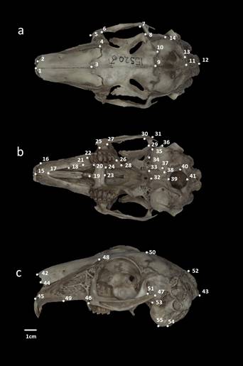
Figure 2 Location of cranial landmarks. a = dorsal view, b = ventral view, and c = lateral view. Voucher specimen the black-tailed jackrabbit (Lepus californicus; CIBNOR 15520) from Todos Santos, Baja California Sur, México, corresponding to group D.
Two separate analyses were conducted using BI. Metropolis-coupled Markov chain Monte Carlo (MCMC) sampling was performed with four chains run for 5 million iterations using default model parameters as baseline values. The sequence evolution model that best fitted each of our sequence datasets was determined using jModeltest ver. 2.1.10 (Darriba et al. 2012) with the Akaike Information Criterion (AIC). Trees were sampled every 1,000th iteration after examining the output files for convergence using the online software AWTY (Wilgenbusch et al. 2004). Majority-rule consensus trees were obtained by summarizing all trees after a burn-in period of 2 million generations. Bayesian probabilities and the frequency of a nodal resolution were taken from the 50 % majority-rule consensus of the trees sampled.
The ingroup included 49 specimens of L. californicus obtained from GenBank (Álvarez-Castañeda and Lorenzo 2017; see Appendix 1) representing the same groups as the geometric morphometrics analysis (Figure 1). Outgroup comparisons used sequences from Sylvilagus audubonii (GenBank accession number KU759759) and S. floridanus (GenBank accession number KU759758).
Results
Morphological Comparison. Specimens from south of Río Nazas (SRN) and north of Río Conchos (NRC) differed in some external morphological characteristics despite having been collected in the same season (Figure 3). SRN specimens had short fur, and the back was whitish-gray; belly was white; a black nape patch extended towards the base of the ears; the tip of the ears had a black patch on the back that extended to the distal edge of the ear; ears were light yellowish-brown on the front with a white outer border (Figure 3). On the other hand, NRC specimens had longer fur and lacked any black stripe on the nape; back was whitish-brown; belly was white; nape patch was light gray; the tip of the ears had a black patch on the back that extended to the distal edge; ears were light brown with whitish hairs on the front of the ears and white outer border (Figure 3). The specimens in the BCP groups A-D show no noticeable differences in pelage coloration; all had medium fur, and the back was blackish-brown mixed with white; belly was yellowish (slightly darker brown in group D); the nape patch was blackish brown and extended towards the base of the ears; the tip of the ears had a black patch on the back that extended to the distal edge of the ear; ears were gray mixed with white on the front with a white outer border (Figure 3).
Somatic measurements are displayed in Table 1. Ear length was slightly shorter in specimens in BCP Groups B, C, and D; hindfoot length also was shorter in Groups C and D. In general, NRC and SRN specimens were larger in body length, hindfoot length, and ear length, relative to BCP specimens (except group A). There were significant differences between NRC and SRN groups in tail length (t-value 2.44, d. f. = 12, P = 0.03). Significant differences (P < 0.05) by t-test values were observed between NRC-SRN and A-D groups in all somatic measurements. In addition, significant differences (P < 0.05) were observed between groups A-D in tail length, hindfoot length, and ear length.
Table 1 Average and ranges (in parenthesis) of somatic measurements of specimens of Lepus californicus from the Altiplano Central (SRN = South Río Nazas; NRC = North Río Conchos) and Baja California Peninsula (Groups A-D), México. n = sample size; lowercase letters represent different sample sizes by group: a (n = 2), b (n = 12), c (n = 10), d (n = 62).
| Group | n | Body length (mm) | Tail length (mm) | Hind foot length (mm) | Ear length (mm) | Weight (g) |
|---|---|---|---|---|---|---|
| SRN | 7 | 620.1 (590-678) | 88.6 (77-95) | 121.1 (111-135) | 146.3 (140-160) | 2,435.7 (2,200-2,600) |
| NRC | 7 | 600.4 (563-650) | 79 (70-89) | 127.6 (115-150) | 147 (138-160) | 2,414.3 (2,100-2,700) |
| Group A | 12 | 521.9 (460-570) | 89.2 (80-102) | 115.3 (102-130) | 153.2 (104-185) | 1,900.0 (1,700-2,100)a |
| Group B | 13 | 528.5 (445-630) | 73.4 (55-100)b | 114.5 (90-150) | 120.5 (70-151) | 2,110.1 (1,800-2,750)c |
| Group C | 19 | 515.1 (480-544) | 89.7 (75-115) | 101.7 (88-110) | 111.6 (90-128) | 1,876.3 (1,350-2,300) |
| Group D | 63 | 500.3 (390-795)d | 81.6 (50-130) | 106.8 (88-125) | 120.3 (102-157) d | 1,876.6 (1,200-4,400) |
Geometric Morphometrics Analyses. The skulls of L. californicus specimens from the Altiplano Central and the Baja California Peninsula were not significantly different in size between sexes (ANOVA of log centroid size, P > 0.05; Appendix 3); therefore, data from both sexes were combined in subsequent analyses. The allometric correction (changes in shape correlated with changes in size) between groups showed a highly significant relationship between skull size and shape in dorsal, ventral, and lateral views of the skull, explaining 6.94 %, 11.39 %, and 8.25 % of the variation, respectively. The main cranial structures related to cranial shape were the parietal region (dorsal view), zygomatic arch (dorsal, ventral, and lateral views), and auditory bullae (ventral view); however, no difference was observed in size and shape between any of the groups analyzed. The first two principal components (PC1 and PC2) of the three cranial views failed to identify the different groups (Figure 4a-c); therefore, the variation in the average shape by group was analyzed. This was confirmed by the broken-stick model that indicated that none of the first five eigenvalues obtained for the three views are significant, indicating that each explains less than the minimal variation of the analysis (Appendix 4).
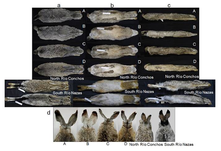
Figure 3 Comparison of external morphology among black-tailed jackrabbit (Lepus californicus) specimens from north Río Conchos (ECO-SC-M 9500), south Río Nazas (ECO-SC-M 9490), and four groups from the Baja California Peninsula (BCP), México: A (CIBNOR 16459); B (CIBNOR 2870); C (CIBNOR 15200); and D (CIBNOR 15508). See Appendix 1 for details of specimens. A-D = groups from the Baja California Peninsula. a = Dorsal view. b = Ventral view. c = Lateral view. d = Nape view.
Relative to the canonical variate analysis (CVA) for the three cranial views, the canonical variate 1 (CV1) was the most useful variate for differentiating between L. californicus from PBC vs. SRN-NRC. The canonical variate 2 (CV2) of the dorsal and lateral views distinguished between NRC and SRN; however, SRN and NRC were not differentiated based on the ventral view (Figure 5a-c).
Skull Dorsal View. The PCA between NRC and SRN indicated that the variation in shape was related primarily to the parietal region, which was higher in NRC and lower in SRN specimens. In contrast, for the BCP group the main differences in the skull concerned the zygomatic arch. The analysis of the continental and peninsular populations combined in PC1 was related primarily to the anterior extension of the zygomatic process, which was larger in NRC-SRN specimens and smaller in the BCP group; PC2 was related to the parietal region, differentiating between NRC (expansion) and SRN (contraction).
The first three canonical variates of the CVA explained 87.7 % of the total variation (Appendix 5). CV1 separated the BCP group from SRN-NRC due to the relative length of the nasals (shorter for SRN-NRC) and the anterior end of the zygomatic process (longer for SRN-NRC). CV2 partially separated SRN from NRC due to the broader inner edge of the orbit, being broader for NRC specimens. The Procrustes distances showed statistically significant differences between NRC and SRN, and between the BCP (except C) and the SRN-NRC groups.

Figure 4 Principal component analysis (PCA) graph, displaying the first two principal components (PC1 and PC2), and deformation grids for PC1 (above) and PC2 (below) for each cranial view of black-tailed jackrabbits (Lepus californicus) specimens: a) dorsal, b) ventral, c) lateral. NRC = north Río Conchos. SRN = south Río Nazas. A-D = groups from the Baja California Peninsula.
Skull Ventral View. The PCA between NRC and SRN indicated that the differences were related to the posterior expansion of the zygomatic arch and the auditory bullae (larger in NRC). The variation in shape was minimal between BCP groups A-D, mainly related to the zygomatic arch and auditory bullae; among the four groups, group C showed the lowest variation. The average variation in shape between continental and peninsular populations associated with PC1 was related to the zygomatic arch and the auditory bullae. SRN-NRC differed from BCP in a smaller zygomatic arch and lateral expansion of the bullae. PC2 discriminated between NRC and SRN due to the smaller bullae in SRN.
In the CVA, the first three factors explained 92.4 % of the total variation (Appendix 5). CV1 (65.2 %) discriminated between SRN-NRC and BCP due to the zygomatic arch and auditory bullae; in CV2 (17.8 %), SRN and NRC overlapped, and no differences were observed. A similar result was detected for the BCP groups A-D. The P values for the Procrustes distances indicated statistically significant differences between SRN-NRC and BCP groups A-D.
Skull Lateral View. The PCA between SRN and NRC indicated that the variation in shape was due to the posterior extension of the zygomatic arch (larger in SRN) and auditory bullae (larger in NRC). The variation in shape in BCP was lower compared to NRC-SRN and was related to the zygomatic arch. The average variation in the shape of the continental and peninsular populations associated with PC1 was related to zygomatic arch length. SRN and NRC had a dorsoventrally shorter zygomatic arch compared to the BCP group. PC2 indicates slight differences between SRN and NRC associated with the relative length of the nasal, which was smaller in NRC.
The first three canonical variates explained 90.2 % of the variation (Appendix 5), CV1 (63.3 %) discriminated between SRN-NRC and BCP due to the dorsoventrally smaller zygomatic arch in SRN-NRC. CV2 (14.4 %) showed a slight overlap between SRN and NRC due to the larger auditory bullae in NRC. The Procrustes distances did not show significant differences between NRC and SRN, but did so between NRC-SRN and BCP (except for group B).

Figure 5 Canonical analysis of variance (CVA) graph, displaying the first two canonical variables (CV1 and CV2), and deformation grids for CV1 (above) and CV2 (below) for each cranial view of black-tailed jackrabbits (Lepus californicus) specimens: a) dorsal, b) ventral, c) lateral. NRC = north Río Conchos. SRN = south Río Nazas. A-D = groups from the Baja California Peninsula.
Discriminant Function Analysis. Assessment of correct classification between pairs of groups by the discriminant function resulted in high allocation percentages (> 92 %) between SRN and NRC and between the different BCP populations for the three cranial views (Table 2). The cross-validation analysis indicated high percentages (83 to 100 %) of correct classification between SRN-NRC and the BCP groups for the ventral and lateral views and low allocation percentages for the dorsal view (45 to 100 %). Regarding the dorsal and lateral views, the incorrect classification of NRC and SRN was 14 % (n = 1) and vice versa, whereas for the ventral view it was 28.57 % (n = 2) and 33.33% (n = 2), respectively. Between NRC and the BCP group, only the ventral view of the skull misclassified 14 % of cases (n = 1). No incorrect classifications were identified between SRN and BCP.
Genetic Analysis. In total, 27 haplotypes for the Cyt b gene were found in 49 sequences (5 SRN, 5 NRC, and 19 BCP; Appendix 1). Eighteen haplotypes were unique: 2 from SRN, 2 from NRC, and 16 from BCP (Table 3). In the Altiplano Central, four haplotypes were shared: two across the rivers between SRN and NRC (haplotypes 4 and 8), one within SRN (haplotype 3), and one within NRC (haplotype 5). The statistical parsimony network of Cyt b (Figure 6b) did not show a clear geographic genetic structure between haplotypes of SRN and NRC. The localities are separated from each other between 1 and 2 mutational steps and they do not share haplotypes with those of BCP group. The haplotypes of BCP group were separated from SRN and NRC by 1 mutational step. The most frequent haplotype was haplotype 9 in seven individuals between groups A and B. In the BCP, five haplotypes were shared among all groups (A to D; haplotypes 9, 17, 19, 24, 26). The Mantel test shows a significant correlation (P < 0.05) between geographic distance and genetic distance between SRN-NRC and for the BCP between A-C and B-D.
Table 2 Percentage of correct assignment for the Lepus californicus groups according to the discriminant function analysis/cross-validation (DFA/CV). See Figure 1 for allocation of localities by group.
| Dorsal cranial view DFA/CV | Group A | Group B | Group C | Group D | North Río Conchos | South Río Nazas |
|---|---|---|---|---|---|---|
| Group A | --- | 100/35 | 100/65 | 100/67 | 100/100 | 100/86 |
| Group B | 100/44 | --- | 88/58 | 93/40 | 100/71 | 100/86 |
| Group C | 100/67 | 95/50 | --- | 87/47 | 100/71 | 100/86 |
| Group D | 100/44 | 95/60 | 85/61 | --- | 100/43 | 100/86 |
| North Río Conchos | 100/100 | 100/45 | 100/88 | 100/80 | --- | 86/43 |
| South Río Nazas | 100/78 | 100/95 | 100/85 | 100/87 | 86/43 | --- |
| Ventral cranial view DFA/CV | ||||||
| Group A | --- | 100/55 | 100/76 | 100/61 | 86/57 | 100/83 |
| Group B | 100/55 | --- | 100/72 | 100/77 | 100/71 | 100/100 |
| Group C | 100/89 | 100/70 | --- | 92/38 | 100/100 | 100/100 |
| Group D | 89/78 | 100/75 | 92/48 | --- | 100/100 | 100/83 |
| North Río Conchos | 100/100 | 100/90 | 92/96 | 100/100 | --- | 67/50 |
| South Río Nazas | 100/100 | 100/100 | 100/100 | 100/100 | 71/43 | --- |
| Lateral cranial view DFA/CV | ||||||
| A | --- | 100/53 | 100/72 | 100/75 | 100/100 | 100/100 |
| B | 100/62 | ---- | 100/72 | 100/75 | 100/100 | 100/100 |
| C | 100/62 | 100/74 | ---- | 92/75 | 100/86 | 100/100 |
| D | 100/62 | 100/68 | 100/56 | --- | 100/86 | 100/86 |
| SRC | 100/100 | 100/100 | 100/92 | 100/100 | --- | 86/57 |
| SRN | 100/100 | 100/95 | 100/96 | 100/83 | 86/57 | --- |
The population with the greatest genetic diversity within-variation was the BCP group D with higher values of H (10), UH (6), P (10), NP (3.25), and π (0.13), followed by BCP group C and SRN (Table 3). Values for the genetic variation parameters of Cyt b are given in Table 3. The average p-distance between individuals from SRN-NRC is 0.8 %, and among all BCP groups was 1.23 % (0.5 to 1.6; Table 4). For populations BCP and NRC, the p-distance was 1.52 % (1.0 to 2.0), and between BCP and SRN, 1.5 % (1.1 to 2.0). The pairwise FST value between NRC and SRN was 0.09; within BCP groups, 0.14 to 0.43; between NRC and BCP groups, 0.43 to 0.58; and between SRN and BCP, 0.39 to 0.56 (Table 4). Statistically significant differences (P < 0.05) were found between specimens from NRC-SRN and BCP (groups A to B).
Table 3 Parameters used for assessing genetic variation of Cytochrome b among groups of Lepus californicus. Abbreviations as follows: total sample size (N); number of haplotypes (H); unique haplotypes per group (UH), number of polymorphic sites (P); number of observed sites with transitions (Tt); number of observed sites with transversions (Tv); mean number of pairwise differences (NP); nucleotide diversity (π); and Fu’s Fs (F). *Indicates significance at P < 0.001.
| N | H | UH | P | Tt | Tv | NP | π | F | |
|---|---|---|---|---|---|---|---|---|---|
| 49 | 27 | 25 | 16 | 9 | 4.110 ± 2.082 | 0.164 ± 0.092 | -17.057 | ||
| Group | |||||||||
| North Río Conchos | 7 | 5 | 2 | 4 | 3 | 1 | 2.000 ± 1.276 | 0.000 ± 0.058 | -1.547 |
| South Río Nazas | 7 | 5 | 2 | 6 | 4 | 2 | 2.190 ± 1.320 | 0.087 ± 0.062 | -1.352 |
| Group A | 3 | 1 | 0 | 0 | 0 | 0 | 0.0 ± 0.0 | 0.0 ± 0.0 | 0* |
| Group B | 8 | 5 | 4 | 8 | 5 | 3 | 2.000 ± 1.256 | 0.080 ± 0.057 | -1.151* |
| Group C | 7 | 5 | 4 | 8 | 8 | 0 | 3.238 ± 1.895 | 0.129 ± 0.086 | -0.552* |
| Group D | 17 | 10 | 6 | 10 | 5 | 5 | 3.250 ± 1.761 | 0.130 ± 0.078 | -3.125* |
The phylogenetic reconstructions used the sequence evolution model TIM3+I+G that best fit our sequence data set. In the BI tree, the Cyt b gene converged on tree topologies that were virtually identical to those of distance and ML (data not shown) analyses. Lepus californicus was found to be monophyletic in the Cyt b gene, with higher bootstrap support (100), and is represented by two subclades (A and B). Subclade A is polyphyletic, including haplotypes of SRN and NRC populations, and subclade B is polyphyletic, including haplotypes of BCP populations (Figure 6a; Appendix 1).
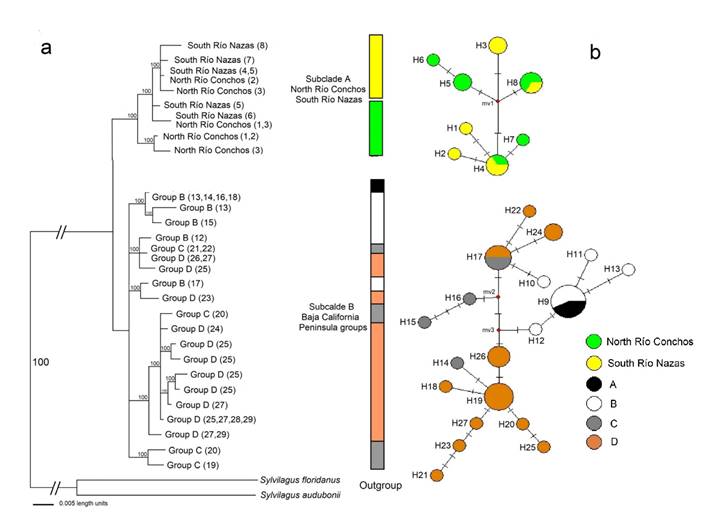
Figure 6 a) Bayesian inference (BI) tree generated by the consensus tree with the 50% majority-rule algorithm of Lepus californicus from north Río Conchos, south Río Nazas and groups of the Baja California Peninsula, based on Cyt b haplotypes. The tip of each branch includes the group and its location number (in parenthesis; see Appendix 1 and Figure 1 for details). Values of branch support are indicated on the phylogenetic tree. b) Haplotype network of 27 non-redundant haplotypes (H) recovered from the Cyt b (625 bp) dataset that included all populations of L. californicus. Transverse lines crossing the lines connecting haplotypes represent the number of base-substitution differences. The size of each circle represents the frequency of the haplotype in the gene.
Table 4 Average genetic p-distances estimated from Cyt b sequences between groups of Lepus californicus (above diagonal) and FST values (below diagonal) for pairs of populations.
| North Río Conchos | South Río Nazas | Group A | Group B | Group C | Group D | |
|---|---|---|---|---|---|---|
| North Río Conchos | - | 0.8 | 1.0 | 1.3 | 1.7 | 2.0 |
| South Río Nazas | 0.09 | - | 1.1 | 1.4 | 1.5 | 2.0 |
| Group A | 0.58 | 0.56 | - | 0.5 | 1.1 | 1.5 |
| Group B | 0.49 | 0.48 | -0.17 | - | 1.4 | 1.6 |
| Group C | 0.43 | 0.39 | 0.35 | 0.32 | - | 1.3 |
| Group D | 0.52 | 0.53 | 0.43 | 0.41 | 0.14 | - |
Discussion
Groups of L. californicus from SRN and NRC did not show statistical differences in size and shape versus any of the other groups analyzed in cranial views. Only minor differences were found in four specific skull regions: 1) parietal (dorsal and ventral views), 2) nasal (dorsal and lateral views), 3) zygomatic arch (dorsal, ventral, and lateral views), and 4) auditory bullae (ventral view). Compared to SRN, the NRC population has an expanded parietal region, reduced nasals, wider zygomatic arch, and more prominent auditory bullae. SRN has a contracted parietal region, wider nasals, narrower zygomatic arch, and less prominent auditory bullae.
It has been postulated that skull variation can be associated with ecological and biological aspects and results from the adaptation to specific environmental, dietary, and physiological pressures (Bowers and Brown 1982; Cox et al. 2012; Klingenberg 2013). The variations in morphology in L. californicus may be related to physiological and nutritional adaptations, making populations capable of inhabiting many types of habitats with diverse ecological and climatic characteristics (Brown et al. 2019). The absence of significant differences between SRN and NRC populations could be considered as a similar adaptation process to the different environments associated with dietary and physiological pressures. Therefore, the genetic differences found between SRN and NRC (0.8 %) are similar or lower than those within BCP populations (0.5 to 1.6 %) without a physical barrier that can restrain the dispersal across populations. On the other hand, the genetic differences between east and west across the Gulf of California are far greater (1.0 to 2.0 %). These findings suggest that the east-west analysis across the Gulf of California-Colorado River reveals a very strong effect, with a greater genetic distance; however, the genetic distance between north and south across the Conchos-Nazas rivers is lower than in the BCP, which lacks a fluvial barrier.
The morphological differences found between SRN and NRC could be more closely related to selective traits that can increase or decrease the predation rate of individuals and as a plastic response to ecological differences (as in small rodents; Neiswenter and Riddle 2010; Neiswenter et al. 2019), such as color pattern variations of the body. Each group was found in a different habitat: SRN in thorn scrubs and savannas and NRC in grasslands. The BCP populations possessed differences in coloration, total size (approximately 20 %), and leg and ear sizes. These characters are associated with semidesert grasslands and scrub vegetation growing in sandy habitats with coastal vegetation (Lorenzo et al. 2010). Therefore, CVA and DFA show differences in the skull between the mainland and peninsular populations, but not within either the mainland or the peninsula.
Also, data from mitochondrial DNA support two distinct genetic groups in the distance, ML, and BI methods. The first includes SRN-NRC specimens with no phylogenetic break associated with barriers such as Río Conchos and Río Nazas; the second comprises BCP specimens and multiple ramifications suggesting a cryptic structure and genetic diversity (Neiswenter et al. 2019) within L. californicus.
Among the specimens of different groups collected throughout BCP (at similar latitudes and with no geographic barriers), the genetic p-distance between their populations was greater (1.23 % on average), as well as the genetic differentiation between groups (0.14 to 0.43; Table 4). The results of the Mantel Test were similar for the population with the presence of the rivers as possible barriers (SRN-NRC) that those which do not have a physical barrier (BCP: A-C and B-D). In the three cases, the genetic distances were significantly correlated with the geographical distance in the same geographical distance (c. a. 600 km) among groups (SRN-NRC, A-C and B-D). It is probable that the evolutionary process in L. californicus has occurred differentially. It may be slower in the Río Conchos and Río Nazas area, so that it is not reflected as a vicariant process. In contrast, evolutionary rates may be faster in BCP, leading to morphological and genetic differences among its populations (Álvarez-Castañeda and Lorenzo 2017).
Four conclusions that can be taken from this study are as follows. A) The canyon system that separates SRN and NRC can limit the gene flow of many species and the dispersal of small mammals (mostly small rodents) and lead to subspeciation, as in S. audubonii and L. callotis; however, it does not seem to be an effective barrier for L. californicus. B) The canyon system in the mainland can be equivalent to the ecological barrier in the BCP (as gene flow between populations is seemingly limited in both cases and the Gulf of California-Rio Colorado barrier is far stronger than that of the Ríos Nazas and Conchos. C) The phenotypic differences between populations may be due to the unique selection pressures in each one, according to their particular distribution occupying different habitats, probably leading to expeditious local adaptations associated with vigorous demographic expansion and probably rapid radiation (Melo-Ferreira and Alves 2018), as suggested by the Fu’s Fs test values for Cyt b. D) The high vagility of L. californicus, favored by changes in land use in addition to its broad distribution range, have probably induced the conditions for a continuous gene flow throughout the Altiplano Central driven by dispersal across the canyon system.

