


 nueva página del texto (beta)
 Inglés (pdf)
 Artículo en XML
 Referencias del artículo
 Enviar artículo por email
 Citado por SciELO
  Similares en
SciELO
Similares en
SciELO 
 Permalink
Introduction
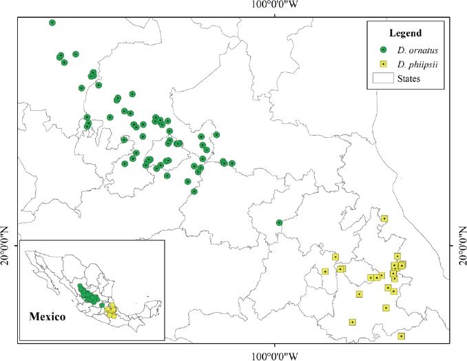
Kangaroo rats Dipodomys ornatus and D. phillipsii are two Nearctic rodents endemic to Mexico, adapted to semi-arid and arid environments. Both taxa are currently distributed across a narrow strip of arid and semi-arid habitats in central-southern Mexico, stretching from southeast Durango (Mexican Plateau, MP) toward southern Puebla and northern Oaxaca (Trans-Mexican Volcanic Belt, TMVB; McMahon 1979; Schmidly et al. 1993). The current taxonomy recognizes D. ornatus at species level (previously D. p. ornatus), and D. phillipsii comprising three subspecies: D. p. oaxacae, D. p. perotensis and D. p. phillipsii (Fernández et al. 2012; Ramírez-Pulido et al. 2014).
Although both species are morphologically similar (Genoways and Jones 1971; Jones and Genoways 1975; Hall 1981; Genoways and Brown 1993), these differ in size, pelage color, and cranial shape (Merriam 1894); also, there are genetic differences and a marked geographical variation between their populations. D. ornatus and D. phillipsii are mid-sized kangaroo rats (total length 245 to 280 mm). Comparing both taxa, northern populations (D. ornatus) are medium to large in size, with pale fur and broad cranium. In contrast, D. p. phillipsii inhabits the Valley of Mexico and adjacent areas, being mid-sized, darker in color, and with a broad interorbital region. The populations of D. perotensis are distributed in Tlaxcala, Puebla, and Veracruz, characterized by larger individuals with fur color intermediate between D. ornatus and D. phillipsii; for its part, D. p. oaxacae, which has been reported in southern Puebla and northern Oaxaca, is the smallest of all subspecies (Jones and Genoways 1975).
These rodents are nocturnal, feeding mainly on seeds, leaves, and small plants. They get metabolic water from the food they eat, living in mound-shaped, gently-sloping burrows with various entrances built in open areas. Both species prefer semi-arid and arid zones with sandy soils and xerophytic vegetation with large grasses (Davis 1944; Hall and Dalquest 1963; Genoways and Jones 1971; Jones and Genoways 1975). Their altitudinal distribution ranges from 950 m a.s.l. in Oaxaca to 2,850 m a.s.l. in Veracruz (Jones and Genoways 1975).
The Mexican authorities in conservation issues (Mexican Official Standard 059) consider D. phillipsii and D. ornatus as a single species (D. phillipsii), listed under the endangered category, and hence subject to protection (SEMARNAT 2010). The first stage in management and conservation plans for threatened or endangered species is to determine their distribution and ecological niche. Grinnell (1917) defined ecological niche as the habitat characterized by environmental conditions that are suitable for population to survive and reproduce. These environmental conditions determine the distribution of a given species.
Predictive species distribution models (SDMs) facilitate the identification of suitable habitats for the conservation of populations, aimed at preventing extinctions. SDMs are based on the correlation between geographic records of species and the respective environmental variables; these kind of data have been used for modeling the potential distribution of species (Elith et al. 2006; Peterson 2006; Kumar and Stohlgren 2009) like a threatened and endangered tree species in New Caledonia, using small number of occurrence records (11).
To date, few studies focus on predicting potential distribution areas for species endemic to Mexico with a distribution restricted to MP and TMVB (Jones and Genoways 1975). Therefore, the objective of this study was to model the ecological niche of two endemic rodents, D. ornatus and D. phillipsii, using MaxEnt to infer potential areas for conservation.
Materials and Methods
Study Area. Presence data were used for Dipodomys phillipsii and D. ornatus in 11 States of Mexico: Aguascalientes, Durango, State of Mexico, Jalisco, Oaxaca, Puebla, Queretaro, San Luis Potosí, Tlaxcala, Veracruz, and Zacatecas (Figure 1), all of which include arid and semi-arid zones (Fernández et al. 2012; Ramírez-Albores et al. 2014). According to presence data for both species, these are distributed in xeric vegetation covering semi-arid and arid zones (Rzedowski 2006); this vegetation includes rosetophilous desert scrub, succulent scrub vegetation, natural grasslands and low deciduous forests, in addition to annual rainfed agricultural crops (INEGI 2016).
The region stretching from Durango to northern Oaxaca comprises various topographic conditions and soil types; those related to kangaroo rat presence data are Kastanozem, Leptosol, Chernosem, Durisol, Phaeozem, Cambisol, Andosol, Arenosol, Regosol, and Vertisol (INEGI 2016). Climate ranges from arid and dry (central-northern Mexico) to temperate and humid (center-south). Mean annual temperature ranges between 12 ºC and 26 °C. The northern part of the country is a desert area, where climate is usually more extreme and with little annual precipitation, which increases southwards (INEGI 2016).
Data sources. A total of 91 presence data were gathered, 63 for D. ornatus and 28 for D. phillipsii, as reported by Fernández et al. (2012), Ramírez-Albores et al. (2014) and obtained from the VertNet database (http://www.vertnet.org/index.html, Esselstyn 2015; Garner 2015; Gegick 2015; Orrell 2015; Prestridge 2015; Revelez 2015; Abraczinskas 2016; Conroy 2016; Cook 2016; Flannery 2016; Opitz 2016; Braun 2017; Gall 2017; Grant 2017; Slade 2017; Feeney 2018, and Millen 2018, Figure 1). Table 1 lists the 27 environmental variables used in the analysis, with a resolution of 30 arc-seconds (pixel size approx. 1 km2), including 19 climatic variables obtained from the WorldClim database (http://www.worldclim.org; Hijmans et al. 2005), three variables on soil properties, three topographical variables, one climate variable, and one variable regarding land use and vegetation; all were obtained from the National Institute of Statistics and Geography of Mexico (INEGI 2015). The latter were selected a priori taking into consideration previous work describing the ecology of the species studied (Merriam 1894; Genoways and Jones 1971; Genoways and Brown 1993).
Table 1 Predictive environmental variables used in the distribution model of kangaroo rats Dipodomys ornatus and D. phillipsii.
| Variables |
|---|
| 1) WorldClim Climate Variables |
| BIO1 = Mean annual temperature |
| BIO2 = Mean diurnal range (maximum temperature - minimum temperature; monthly average) |
| BIO3 = Isothermality (BIO1/BIO7) * 100 |
| BIO4 = Temperature seasonality (coefficient of variation) |
| BIO5 = Maximum temperature of the warmest period |
| BIO6 = Minimum temperature of the coldest period |
| BIO7 = Annual temperature range (BIO5-BIO6) |
| BIO8 = Mean temperature of the wettest quarter |
| BIO9 = Mean temperature of the driest quarter |
| BIO10 = Mean temperature of the warmest quarter |
| BIO11 = Mean temperature of the coldest quarter |
| BIO12 = Annual precipitation |
| BIO13 = Mean precipitation of the wettest period |
| BIO14 = Mean precipitation of the driest period |
| BIO15 = Precipitation seasonality (coefficient of variation) |
| BIO16 = Mean precipitation of the wettest quarter |
| BIO17 = Mean precipitation of the driest quarter |
| BIO18 = Mean precipitation of the warmest quarter |
| BIO19 = Mean precipitation of the coldest quarter |
| 2) Soil Properties |
| HUM = Soil moisture |
| SUELOTY = Soil type |
| TEXT = Soil texture |
| 3) Topographic Variables |
| SLOPE = slope |
| TOPO = Topoforms |
| CEM = Mexican elevation continuum |
| 4) Type of Climate |
| CLIM = Climate Units |
| 5) Land Use and Vegetation |
| USES = Land use and vegetation |
Modeling. First, a randomness test was run with the georeferenced records of each species (D. ornatus and D. phillipsii) using the R statistical package (R Development Core Team 2018). The randomness test determines whether records are spatially distributed at random or clustered (Bivand et al. 2008). If data are not clustered, 75 % of records are used as training data, and the remaining 25 %, as testing data. For clustered data, a pattern analysis is conducted to estimate the probability of finding one record at a certain distance, expecting no spatial autocorrelation between data (Hengl 2007). The pattern analysis is run with the ILWIS 3.3 software (https://52north.org/software/software-projects/ilwis/). If the pattern analysis confirms clustered data, the software ArcGis v9.2 (ESRI 2006) randomly selects 50 % of the total number of records, which are used for model training, and the rest are used for model validation.
From the 27 climate variables in raster data files, a Principal Component Analysis (PCA) was run to avoid multicollinearity — a statistical issue defined as a high degree of correlation between variables. When variables are highly correlated, small changes in data or variables may lead to considerable changes in the distribution of species; consequently, estimates from the resulting models are unreliable (Quinn and Keough 2002). Using the R statistical package, these data were described as a group of new variables (components) that were not correlated with each other. Eleven principal components (PC, raster data files) were used as new environmental variables, which accounted for over 95% of the variance of the original variables.
SDMs of the rodents studied were constructed using the MaxEnt software (https://biodiversityinformatics.amnh.org/open_source/maxent/), which requires geographic presence records (which is an advantage for the modeling of endemic species with small populations and scarce records; Phillips et al. 2006), and a set of climatic and/or ecological variables that are part of the information about the known distribution of species. This software works with a limited number of samples and climatic variables (topography, climate, soil type, Papeş and Gaubert 2007; Pearson 2007; Hernandez et al. 2008; Phillips and Dudik 2008; Wisz et al. 2008), as well as categorical and continuous variables, requiring knowledge about the biology of the species for the correct interpretation of results (Elith et al. 2006). In addition, it provides a continuous result and analyses are repeatable (Phillips et al. 2006; Phillips and Dudik 2008).
The parameters used for modeling were those displayed by default by MaxEnt version 3.3.3k, except for the "Extrapolate" and "Do clamping” parameters, which were disabled; the data output was logistic. The models obtained were validated using a cut-off threshold value equal to the maximum test sensitivity plus specificity (Liu et al. 2005), which maximizes the cases where the model erroneously assigns an unsuitable habitat (true negative) and ignores the suitable habitat (false positive); this approach is very common when using MaxEnt (Ferraz et al. 2012; Jorge et al. 2013; Kebede et al. 2014). In addition, we conducted a preliminary validation by calculating the area under the curve (AUC = Area under a Receiver Operating Characteristic [ROC] Curve). The AUC ranges from 0 to 1; an AUC of 0.5 indicates that this model is not better than one constructed at random, while a value of 1 indicates a perfect fit of the model (Pearce and Ferrier 2000; Newbold et al. 2009). Subsequently, a binomial test was performed, which evaluates whether the model obtained is better than one derived at random (p > 0.5) based on omission rates (i.e., proportion of test records that fall outside of the predicted area, considering cut-off threshold). Successful records are those with logistical values above the selected cut-off threshold (Elith et al. 2011; Cruz-Cárdenas et al. 2014). Finally, the models obtained with the MaxEnt algorithm were reclassified into Boolean layers (presence/absence), using the cut-off threshold. MaxEnt produces logistic data, i.e., continuous values ranging from 0 to 1 that represent the probability of occurrence of the species in the area, and which are represented on a map (Bean et al. 2014). Data were reclassified using the software ArcGis v9.2 (ESRI 2006; Pliscoff and Fuentes-Castillo 2011). Some previous studies of threatened species (Aguilar-Soto et al. 2015; Rovzar et al. 2013) established ranges of probability of occurrence based on the distribution of species. The 0.7 to 1 range indicates high probability of occurrence, where most geographic records are located; 0.5 to 0.7 indicates medium probability, including the remaining records; and finally threshold to 0.5 represents low probability of occurrence. These probability ranges have been used in ecological studies for various species (Bailey et al. 2002; Woolf et al. 2002; Liu et al. 2005; Gil and Lobo 2012; Martínez-Calderas et al. 2015). To calculate the area (km2) predicted by models, the number of pixels belonging to each classification was counted and multiplied by 30 arches-seconds (pixel resolution) for each probability of occurrence (low, medium, and high).
Results
The randomness analyses of geographic records of both species reveals a clustered pattern; Figure 2 shows that values (solid line, G^obs[r]) lie outside the confidence interval (gray area G^hi[r] and G^o[r]) estimated by distance (r). If the solid line (G^obs[r]) lies within the upper and lower lines (G^hi[r] and G^o[r]), the data are statistically distributed at random, with no cluster pattern. If G^obs[r] is located outside of these confidence lines, it indicates a spatial pattern, i.e., data are clustered. The records for D. ornatus (Figure 2A) show a clustering pattern, where the probability of finding another record is G(r) = 0.9 at a distance of 33 km (r = 0.3 degrees). On the other hand, the records for D. phillipsii (Figure 2B) show a lower clustering pattern, with a probability of finding another record G(r) = 0.8, although these involve a distance of 22 km (r = 0.2 degrees).
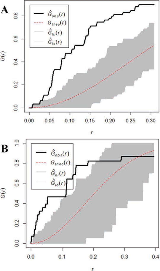
Figure 2 Randomness analysis of geographic records. A) Dipodomys ornatus, and B) Dipodomys phillipsii. The dotted line corresponds to calculated theoretical values, the gray area corresponds to the confidence interval, and the solid line corresponds to observed values in our data.
The pattern analysis of geographical records of both species with the software ILWIS 3.3 resulted in the selection of 8 of 63 records for D. ornatus for model training, and 4 of 28 records for D. phillipsii. To validate the model, 12 test records were selected at random for D. ornatus, and 6 for D. phillipsii. When the potential distribution model was constructed for both species, these did not pass the binomial test validation; hence, the models obtained are not better than one obtained at random (P > 0.5). Consequently, all records were splitted in 50 % for model training plus 50 % for model validation for both species. The PCA of the 27 climatic variables produced 11 PCs that altogether account for 95 % of the variability of the original variables. The environmental variables with the highest contribution in the 11 PCs used are listed in Table 2, taking into account the loading factors.
Table 2 Contribution of environmental variables used in the Principal Component Analysis (Loading factors) for kangaroo rats Dipodomys ornatus and D. phillipsii.
| Original variables | PC1 | PC2 | PC3 | PC4 | PC5 | PC6 | PC7 | PC8 | PC9 | PC10 | PC11 |
|---|---|---|---|---|---|---|---|---|---|---|---|
| bio1 | -0.219 | 0.290 | -0.098 | 0.008 | -0.053 | 0.047 | -0.021 | -0.007 | 0.030 | 0.017 | -0.046 |
| bio2 | 0.242 | -0.032 | -0.110 | 0.175 | 0.063 | -0.242 | 0.131 | -0.016 | 0.134 | -0.535 | -0.154 |
| bio3 | -0.156 | -0.196 | -0.344 | -0.182 | -0.071 | -0.070 | -0.011 | 0.002 | 0.157 | -0.385 | -0.044 |
| bio4 | 0.222 | 0.187 | 0.271 | 0.214 | 0.067 | -0.029 | 0.064 | -0.018 | -0.083 | 0.094 | -0.021 |
| bio5 | -0.024 | 0.393 | 0.005 | 0.190 | 0.005 | -0.067 | 0.040 | -0.029 | 0.026 | -0.192 | -0.139 |
| bio6 | -0.281 | 0.139 | -0.131 | -0.127 | -0.071 | 0.097 | -0.087 | -0.010 | 0.024 | 0.025 | 0.000 |
| bio7 | 0.268 | 0.104 | 0.135 | 0.246 | 0.074 | -0.140 | 0.112 | -0.008 | -0.008 | -0.144 | -0.086 |
| bio8 | -0.107 | 0.334 | 0.011 | 0.209 | -0.020 | -0.010 | 0.099 | 0.035 | 0.023 | 0.183 | -0.025 |
| bio9 | -0.213 | 0.231 | -0.157 | 0.018 | -0.003 | 0.020 | -0.059 | -0.050 | 0.057 | -0.339 | -0.101 |
| bio10 | -0.089 | 0.396 | 0.042 | 0.124 | -0.011 | 0.041 | 0.005 | -0.021 | -0.017 | 0.029 | -0.078 |
| bio11 | -0.269 | 0.146 | -0.205 | -0.091 | -0.067 | 0.055 | -0.051 | -0.003 | 0.060 | -0.058 | -0.035 |
| bio12 | -0.281 | -0.133 | 0.090 | 0.156 | -0.008 | -0.036 | 0.066 | 0.012 | 0.008 | -0.065 | 0.065 |
| bio13 | -0.264 | -0.142 | -0.013 | 0.275 | 0.028 | -0.001 | 0.114 | 0.026 | -0.021 | -0.005 | 0.097 |
| bio14 | -0.228 | -0.059 | 0.369 | -0.031 | -0.013 | -0.155 | -0.034 | -0.035 | 0.025 | -0.102 | 0.041 |
| bio15 | 0.046 | -0.054 | -0.409 | 0.429 | 0.135 | 0.018 | 0.241 | 0.111 | 0.006 | 0.037 | 0.060 |
| bio16 | -0.262 | -0.153 | -0.029 | 0.262 | 0.017 | -0.002 | 0.121 | 0.030 | -0.007 | -0.021 | 0.085 |
| bio17 | -0.227 | -0.064 | 0.380 | -0.022 | -0.010 | -0.146 | -0.039 | -0.054 | 0.016 | -0.104 | 0.068 |
| bio18 | -0.211 | -0.145 | 0.016 | 0.344 | 0.095 | -0.028 | 0.164 | -0.007 | -0.076 | 0.133 | 0.217 |
| bio19 | -0.206 | -0.061 | 0.357 | 0.064 | 0.041 | -0.080 | -0.067 | -0.144 | 0.002 | -0.326 | 0.071 |
| CEM | 0.156 | -0.339 | -0.048 | 0.013 | -0.002 | -0.110 | 0.059 | 0.044 | 0.052 | -0.020 | 0.029 |
| CLIM | -0.242 | -0.139 | -0.106 | 0.020 | -0.041 | -0.024 | 0.054 | 0.140 | 0.043 | 0.212 | -0.080 |
| HUM | -0.113 | -0.198 | 0.202 | 0.058 | 0.071 | 0.178 | 0.102 | 0.243 | 0.270 | 0.120 | -0.812 |
| SLOPE | -0.012 | -0.188 | -0.095 | 0.264 | -0.074 | 0.244 | -0.409 | -0.300 | -0.653 | -0.104 | -0.309 |
| SUELOTY | -0.044 | -0.001 | -0.099 | 0.071 | 0.756 | -0.142 | -0.515 | -0.149 | 0.279 | 0.139 | 0.012 |
| TEXT | 0.084 | -0.086 | -0.039 | 0.245 | -0.453 | -0.017 | -0.118 | -0.632 | 0.511 | 0.199 | -0.030 |
| TOPO | 0.070 | 0.004 | 0.010 | 0.281 | -0.380 | -0.213 | -0.590 | 0.590 | 0.109 | -0.007 | 0.093 |
| USES | -0.111 | 0.024 | -0.153 | -0.126 | -0.072 | -0.819 | 0.073 | -0.124 | -0.280 | 0.253 | -0.267 |
PC = PCA principal component. The loading factors of original variables are highlighted in black.
At this scale level, for the distribution model of D. ornatus, PC2, PC11, and PC1 had the highest contribution to the probability of occurrence of the species (68.2 %; Table 3). For the distribution model of D. phillipsii, PC4, PC2, and PC6 made the highest contribution to the probability of occurrence of the species (80.14%; Table 3). The variables maximum temperature of the warmest period (BIO5), mean temperature of the wettest quarter (BIO8), and mean temperature in the warmest quarter (BIO10) are elements of the PC with the highest contribution to the predictive distribution model for D. ornatus. For their part, seasonality of precipitation (BIO15), precipitation in the warmest quarter (BIO18), and topography (TOPO) are the variables with the greatest influence in the distribution model of D. phillipsii.
Table 3 Percent contribution of the main components resulting from MaxEnt models for kangaroo rats Dipodomys ornatus and D. phillipsii. The most important principal components for each species are highlighted in bold.
| D. ornatus | D. phillipsii | |
|---|---|---|
| PC1 | 17.7 | 0 |
| PC2 | 30.6 | 21.0 |
| PC3 | 11.5 | 3.3 |
| PC4 | 5.8 | 58.2 |
| PC5 | 0.7 | 4.9 |
| PC6 | 4.5 | 9.4 |
| PC7 | 2.2 | 0 |
| PC8 | 2.7 | 0 |
| PC9 | 0.8 | 1.9 |
| PC10 | 3.5 | 1.9 |
| PC11 | 19.9 | 0 |
Figure 3 shows the omission rates and predicted area for both species. The calculated omission rates are expected to be close to the predicted omission rates (black line). Figure 3A shows that the omission rate of the calculated test records are close and above the predicted omission data; thus, it can be considered that the test records used for the model of D. ornatus are not spatially autocorrelated, and can be considered as an appropriate model. By contrast, Figure 3B, for the model of D. phillipsii, shows that the omission rate of the calculated test records is close to but below the predicted omission values, indicating that the training and test records are not independent and are spatially autocorrelated, due to the number of records used for training and testing, in addition to the clustering pattern of these records (Phillips et al. 2006).
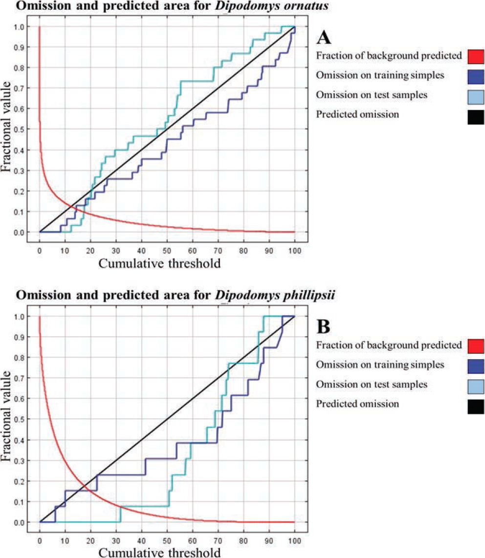
Figure 4 shows the predicted distribution model for D. ornatus and the areas of occurrence predicted by this model. The cut-off threshold value selected was 0.173 (maximum test sensitivity plus specificity; Liu 2005). Predicted distribution areas were classified into low (0.173 to 0.5), medium (0.5 to 0.7), and high (0.7 to 0.951) probability of occurrence. The model shows an AUC = 0.963 for training data and an AUC = 0.954 for test data, with a standard deviation of 0.0068. This cut-off threshold was associated to an omission rate of test records equal to 0. The model shows that the predicted distribution area for this species is concentrated in the central region of Mexico in mostly dry climates, distributed across the States of Durango, San Luis Potosí, Zacatecas, Aguascalientes, Guanajuato, Querétaro, and Hidalgo. The predicted low, medium and high probability areas (green, yellow and red, respectively) were approximately 197,488 km2, 30,894 km2, and 20,927 km2 (Figure 4).
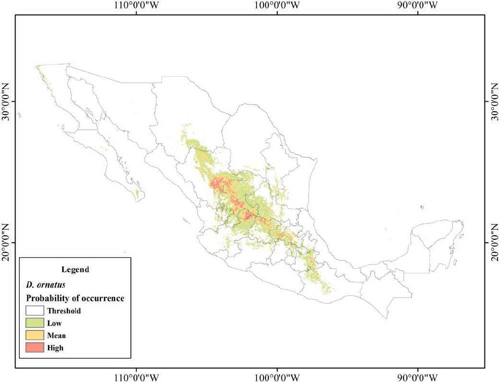
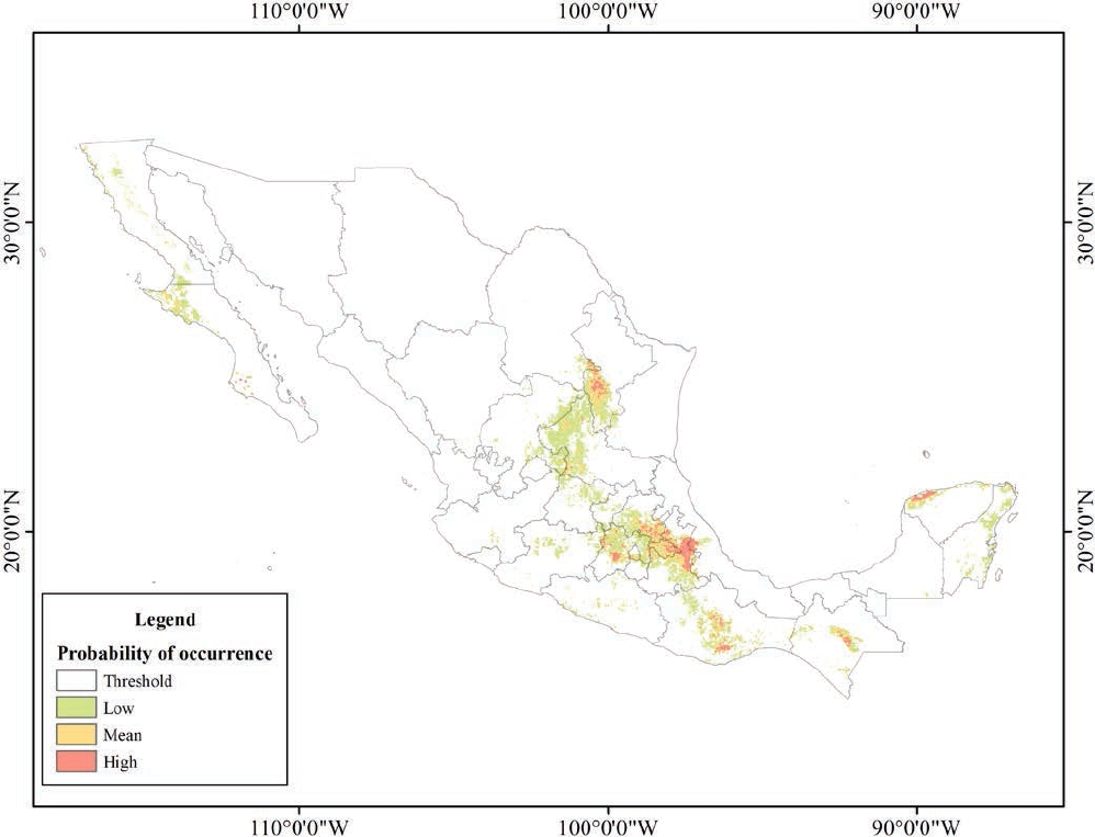
Figure 5 shows the predicted distribution model for D. phillipsii and the areas of occurrence predicted by this model. The cut-off threshold value of the maximum test sensitivity plus specificity was 0.248. Similar to the model for D. ornatus, the predicted distribution areas were classified into low (0.173 to 0.5), medium (0.5 to 0.7), and high (0.7 to 0.987) probability of occurrence. The model shows an AUC = 0.930 for training data and an AUC = 0.987 for test data, with a standard deviation of 0.0053. This cut-off threshold was associated to an omission rate of test records equal to 0. The model shows that the predicted distribution area for this species is concentrated in the southern region of the country, particularly in the States of Puebla, Veracruz, Tlaxcala, Hidalgo, and the State of Mexico. Other areas with high a probability of occurrence are the southwestern part of the State of Nuevo León, center-south of Oaxaca, Chiapas, and center-north of Yucatan. The predicted low, medium and high probability areas (green, yellow and red, respectively) were approximately 115,203 km2, 30,894 km2, and 15,944 km2 (Figure 5). Finally, the binomial test determined that the predictive distribution models for both species were better than random models (P > 0.5).
Discussion and Conclusions
Species distribution is determined by the availability of habitat with suitable environmental conditions, in addition to physical barriers such as rivers, mountains and topography that restrain their dispersal, as well as stochastic and anthropological processes (Wiser et al. 1998). Currently, mammals and other taxa are threatened due to multiple factors, including the loss of habitats associated to changes of land use from natural vegetation to cropland and human settlements, resource overexploitation, and climate change (Stuart et al. 2004; Thomas et al. 2004).
It is broadly acknowledged that endemic taxa are particularly susceptible to extinction, as a result of their restricted distribution, specificity of habitat and habits, and high vulnerability to environmental changes due to their low genetic variability, which reduces their ability to respond to selective pressures (Isik 2011). The geographical distribution of a species derives from three factors: biotic (preys, competitors, and predators), geographical space available for a species, and environmental conditions where a population can survive (fundamental niche, Maguire 1973). However, some of these conditions may also be found in adjacent areas, representing suboptimal sites where individuals of a species can spread to (Hutchinson, 1957; 1978, Soberón and Peterson 2005). For this reason, predictive species distribution models are an important tool in the analysis of potential habitats; however, this is a limited tool for species with restricted ranges, unique environmental requirements, and limited geographic records, thus restraining their monitoring and conservation (Rhoden et al. 2017), as is the case of some rodents. It should be noted that predicting the distribution of a suitable habitat of a species requires understanding its interactions in addition to the environmental variables in areas of occurrence (Baldwin 2009; Adhikari et al. 2012). For improving the conservation status of the species, potential area and habitat for reintroduction were predicted using Maximum Entropy (MaxEnt).
The MaxEnt models at national level showed an adequate performance in estimating the potential distribution of D. ornatus and D. phillipsii, yielding AUC values of 0.963 and 0.987, respectively; also, both models were validated by a binomial test and an analysis of omission rates. Although the records selected for both species showed a clustering pattern, as these failed the randomness test, these met the statistical requirements for final validation.
A key aspect is to determine that the environmental variables used for modeling are not spatially correlated; otherwise, the models obtained will tend to predict areas with a smaller surface, i.e., the likely area of occurrence of a species is underestimated (Cruz-Cárdenas et al. 2014). For this reason, the environmental variables used should not be spatially correlated; alternatively, the dimensionality of variables should be reduced through statistical analyses such as PCA, which yields PCs that are projections with no correlation with the original variables. This type of statistical analysis should be used on climatic variables such as temperature and precipitation, as is the case of the WorldClim climate variables (Phillips et al. 2006).
The area with a high probability of occurrence, defined by environmental conditions that are favorable for D. ornatus, is situated mainly in the central region of Mexico, where the MP and the Chihuahuan Desert are located, both being areas with dry climate and extreme temperatures. By contrast, the potential distribution areas modeled for D. phillipsii are located mainly at TMVB and SMO, where environmental conditions are wetter with more stable temperate temperatures (INEGI 2016). This indicates habitat preferences of each species; however, it should be stressed that the areas predicted by SDMs are highly correlated with the geographical records used.
The predictive model for D. phillipsii yielded a high probability of occurrence in the south-west of the State of Nuevo León, in an area near the SMO covered by coniferous forest where this species has not been reported. In general, to validate and define the actual distribution of both species, field surveys should be conducted in areas with a probability of occurrence greater than or equal to 0.7. Suboptimal areas showing a probability of occurrence of 0.5 or above may be used as potential shelters in conservation strategies. These rodents are hard to capture given their restricted distribution, and SDMs can contribute to identify potential sampling areas.
Although these species are distributed in several States across the country, only some collection sites have been described in detail; consequently, the ecology of these species and their differences in habitat preference at the local level are poorly known. In general, both species live at altitudes between 950 and 2,850 m a.s.l., in sandy soils covered by low grasslands in association with different cactus species, including prickly-pear cacti, and low thorny shrubs; however, both have specific distribution requirements at a local level.
Dipodomys ornatus inhabits mainly flat deserts with dry climate covered by grasslands and shrubs; the areas of low and medium probability of occurrence obtained with the SDM match these habitats. The areas with a high probability of occurrence correspond to a semidry climate, mainly in natural grasslands of the Chihuahuan Desert and areas with low precipitation and soil moisture, corresponding to MP States (Durango, Zacatecas, San Luis Potosí, and Querétaro; INEGI 2016; CONAGUA 2016). More specifically and according to the literature, southwest to the city of San Luis Potosi, D. ornatus lives near low hills adjacent to oak forests (Dalquest 1953); in Durango, D. ornatus inhabits intermontane valleys covered with low grasslands, thorny shrubs (Mimosa monancistra), and cacti (Opuntia; Jones and Genoways 1975); in Zacatecas, specimens have been collected in areas with volcanic soils, in plains near hills with volcanic rocks, which during the past decade have been used for agricultural crops, forcing D. ornatus to survive in the edges of corn fields (change of land use and vegetation).
By contrast, D. phillipsii was captured in flat, desert habitats with temperate climate and sandy soils covered with shrubs and cacti; sites where this species has been recorded usually have either temperate-humid or warm-humid climate (INEGI 2016). In the States of Hidalgo, Puebla, Tlaxcala, State of Mexico, and Veracruz, the climate is humid due to proximity to the Gulf of Mexico and high precipitation (800-3,000 mm; CONAGUA 2016). Areas of high probability of occurrence, such as the Oriental Basin, where the natural vegetation has been replaced by maize crops (INEGI 2016), match collection sites where Genoways and Jones (1971) collected some specimens. In Veracruz, D. phillipsii is located in open, semi-arid areas covered by shrubs, cacti and agave, with wet climate (Hall and Dalquest 1963); in the State of Mexico and Hidalgo, D. phillipsii inhabits mainly semi-arid valleys covered by grasslands and surrounded by pine-oak forest; in Tlaxcala, specimens of D. phillipsii have been collected within maize crop fields (pers. obs. J. A. Fernandez).
Since the geographical records of the rodents studied are concentrated in MP, the Chihuahuan Desert and TMVB, the variables with the greatest influence in PCs were those related to temperature and precipitation. As observed from SDMs, D. ornatus and D. phillipsii show particular habitat preferences. These models, influenced by the geographical records and environmental variables used, in addition to the genetic evolution and the appearance of physical barriers such as the TMVB, and the multiple physiographic regions of Mexico that act as barriers that isolate geographically and genetically populations of these species, result in the differentiation of two groups defined by their geographical distribution and genetic identity, supporting the taxonomic proposal of Fernández et al. (2012). It is proposed that the altitude of the MP produces conditions that differ from those in high intermontane valleys of TMVB, resulting in two different potential distribution models influenced by different PCs and environmental variables.
Understanding how extrinsic factors influence the distribution of species and the selection of future habitats is key for researchers (Baldwin 2009). These questions can be solved with the assistance of SDMs, as these can provide useful information for the survey and prediction of areas with suitable conditions for the dispersal of species with a restricted distribution (Elith et al. 2011). In addition, SDMs allow the a priori selection of potential sampling areas, thus reducing costs and effort (Fois et al. 2015). It is concluded that MaxEnt is a valuable tool to describe and locate favorable areas for the expansion of populations of endemic species, or to describe more clearly the actual distribution of species in future research.

