


 text new page (beta)
 English (pdf)
 Article in xml format
 Article references
 Send this article by e-mail
 Cited by SciELO
  Similars in
SciELO
Similars in
SciELO 
 Permalink
Introduction
The genus Coendou Lacépède, 1799 (Rodentia: Erethizontidae), distributed only in America, groups together 13 species that live in tropical, subtropical and temperate areas in wet and dry forests, from sea level up to 3,650 masl (Voss et al. 2013; Voss 2015; Brito and Ojala-Barbour 2016). The stump-tailed porcupine Coendou rufescens Gray, 1865 is distributed in the Andes of Colombia, Ecuador and northwestern Peru (Alberico et al. 1999; Voss 2011, 2015; Tirira 2016; Brito and Ojala-Barbour 2016; More and Crespo 2016; Romero et al. 2018). An unusual record from northern Bolivia has been recently reported, representing a biogeographical enigma that suggests that some individuals of this species moved to this area (Voss 2011).
Coendou rufescens is characterized mainly by a short non-prehensile tail, unlike other long-tailed porcupines, in addition to its distinctive reddish coloration (Voss 2015). Although the ecological information available for C. rufescens is rather limited, it is considered as a species that inhabits only mature and well-preserved forests (Tirira 2017). Some point observations in the Sangay National Park in Ecuador have served to characterize the species as either solitary or gregarious (1 to 4 individuals), diurnal and nocturnal (Brito and Ojala-Barbour 2016). Incidental records have documented that the stump-tailed porcupine is preyed upon by pumas (Tirira 2016) and ocelots (Sanchez et al. 2008).
A predictive distribution model can be used to locate suitable or potential habitats outside of the known range of a given species (e. g., Morueta-Holme et al. 2010; Chatterjee et al. 2012; Ortega-Andrade et al. 2015). Some potential-distribution correlation models (Braunisch et al. 2008; Peterson et al. 2011) use information on the current distribution of the species and assume that the habitat where records are located represents the ideal habitat for the species. However, the distribution of many vertebrates (especially those threatened) has shrunk, and thus these species could be considered as refugee species, that is to say, limited to survive in suboptimal habitats due to anthropogenic pressures (Kerley et al. 2012).
One of the methods frequently used for modeling the potential distribution is maximum entropy modeling (e. g., Phillips et al. 2006; Phillips and Dudik 2008; Elith et al. 2011; Renner et al. 2013; Nuchel et al. 2018), which has proved to be useful for establishing high-diversity, high-endemism and conservation areas for vertebrates in Neotropical regions (Cuesta et al. 2017; Reyes-Puig et al. 2017). This method is often better than traditional statistical approaches and other species-distribution modeling methods (Elith et al. 2006; Phillips et al. 2006). However, several authors suggest using a consensus of models to reduce the uncertainty of predictions derived from individual models (e. g., Marmion et al. 2009; Qiao et al. 2015; Zhu and Peterson 2017).
This work reports 10 new localities for Coendou rufescens in Ecuador. A potential distribution model was developed for Colombia, Ecuador and Peru using the new localities, those available in the literature, and those associated to museum vouchers. In addition, the geographical layers of remnant vegetation in the three countries were overlaid and the proportion of each within the potential distribution range was calculated. The information on the extension of the distribution range may be valuable for further taxonomic, phylogenetic and ecological studies, while contributing relevant data for the protection of this poorly known species.
Materials and Methods
Records of living and road killed individuals were obtained through direct field observations during various faunal surveys conducted as part of environmental studies for mining and power companies between years 2007 and 2017. In addition, two specimens of C. rufescens (MEPN 3260 and 10433) deposited in the mammal collection of the Escuela Politécnica Nacional (MEPN), Quito-Ecuador, were also examined. Each encounter was georeferenced and photographed, recording the behavior of each living specimen. In addition, informal interviews were carried out to residents living in the study area to determine the extent of the local knowledge about the species.
Potential Distribution Model. In order to estimate the potential distribution of C. rufescens, records were obtained from the published literature (Gray, 1865; Williams 2008; Ramírez-Chávez et al. 2008; Tirira and Boada 2009; Fernández de Cordoba-Torres and Nivelo 2016; More and Crespo 2016; Brito and Ojala-Barbour 2016; Romero et al. 2018), along with the new records from this study (Appendix 1). Presence coordinates were transformed to the decimal degree coordinate system, Datum WGS84 and Universal Transverse Mercator projection (UTM), zones 17S and 18S. Duplicate coordinates and those that were less than 2 km away from each other were discarded, thus avoiding oversampling presence records while preserving the independence between localities and bioclimatic variables.
The potential-distribution exploratory model was developed based on the 19 bioclimatic variables of WorldClim 19 1.4 (http://www.worldclim.org; Table 1), which are geo-environmental layers derived from monthly temperature and precipitation data with a resolution of ca. 1 km2 (Hijmans et al. 2005). The model was developed with the software MaxEnt v3.3.3 (Phillips et al. 2006) based on the maximum entropy principle and the convergence of environmental variables covering an area of suitable habitat (Elith et al. 2006; Phillips et al. 2006; Ortega-Andrade et al. 2015). The maximum entropy model uses a confusion matrix that combines the predicted presence/absence with pseudo-absence and true-presence data, producing commission and omission rates. In addition, the probability distributions estimated by the software should be consistent with the known environmental conditions of the species (Peterson et al. 2011).
Table 1 Contribution of 19 bioclimatic variables to the predictive model of Coendou rufescens.
| Code | Contribution | Variable |
|---|---|---|
| BIO4 | 28.15 | Seasonal temperature |
| BIO6 | 16.89 | Minimum temperature of the coldest month |
| BIO18 | 15.04 | Precipitation of the warmest annual quarter |
| BIO8 | 10.94 | Mean temperature of the wettest annual quarter |
| BIO19 | 4.72 | Precipitation of the coldest annual quarter |
| BIO11 | 4.64 | Mean temperature of the coldest annual quarter |
| BIO3 | 3.45 | Isothermality |
| BIO10 | 3.22 | Mean temperature of the warmest annual quarter |
| BIO1 | 2.49 | Mean annual temperature |
| BIO14 | 2.38 | Precipitation of the driest month |
| BIO13 | 1.89 | Precipitation of the wettest month |
| BIO7 | 1.64 | Annual temperature range (BIO5-BIO6) |
| BIO16 | 1.32 | Precipitation of the wettest annual quarter |
| BIO17 | 1.25 | Precipitation of the drieest annual quarter |
| BIO15 | 0.52 | Seasonal precipitation |
| BIO12 | 0.45 | Annual precipitation |
| BIO2 | 0.45 | Diurnal mean range (monthly average (max temp-min temp) |
| BIO5 | 0.29 | Maximum temperature of the warmest month |
| BIO9 | 0.18 | Mean temperature of the driest annual quarter |
A total of 52 validated presence records and the 19 bioclimatic variables were entered in MaxEnt. Fifty replicates were run with a Jackknife test to measure the percent contribution of the variables to the model (Phillips et al. 2006; Lizcaino et al. 2015; Ortega-Andrade et al. 2015). A correlation matrix was elaborated with the key variables; highly correlated variables were eliminated by means of a correlation chart (r > 0.8). To build the model, we established a convergence threshold of 0.00001, a maximum of 1000 interactions, and a regularization parameter of 1. The model was tested and calibrated with 50 additional replicates using non-correlated climatic variables; data were split into 25 % as test and 75 % as training data (Menendez-Guerrero and Graham 2013). The “Equal training sensitivity and specificity” cohort threshold was selected, as it reflects a lower omission rate (Liu et al. 2005).
The predictive capacity of the model was evaluated by ROC (Receiver Operating Characteristic) curves and AUC (Area under the Curve) curves (Hanley and Mc Neil 1982; Lobo et al. 2008). In addition, we used the partial area under the ROC curve test (Lobo et al. 2008), thereby avoiding the improper calculation of the weight in AUC commission and omission rates (Lobo et al. 2008; Peterson et al. 2008). Partial AUCs were calculated using the ToolBox developed by Osorio-Olvera (2018). The statistical significance of AUC was tested by bootstrapping and comparisons vs. null hypotheses (i. e., Ho = difference between model-predicted AUC and random AUC is ≤ 0). We used 50 % of presence data at random for the resampling, with 500 iterations. Significance was evaluated using the calculated AUC values and the values of pseudo-replicates following the proposal of Peterson et al. (2008). All distribution, normality and correlation statistical analyzes of variables were run in the statistical program R (R Core Team 2016). Once the model was calibrated, a final model was constructed with 100 % of the presence data and non-correlated bioclimatic variables in order to obtain the distribution predictive model.
The total potential distribution area was calculated for Colombia, Ecuador and Peru (Datum WGS84 and Universal Transverse Mercator (UTM) projection, zones 17S and 18S). In addition, the layers of remnant vegetation (i. e., plant cover of natural ecosystems) and protected areas for the three countries were overlaid to assess the reduction in the distribution of C. rufescens in non-protected areas with no vegetation cover. Maps and calculations of geographic layers were elaborated in ArcMap 10.5.1 (ESRI 2017). The layers of remnant vegetation for Ecuador were obtained from the Sistema Nacional de Información (National Information System) website (SIN 2017); for Colombia, from the Sistema de Información Ambiental de Colombia (Environmental Information System, SIAC 2017); and for Peru, from the Ministry of the Environment´s official website (MINAM 2017).
Results
New localities. In addition to the Ecuadorian localities previously reported in the literature (Appendix 1), the following are the new localities where the species has been spotted.
1) Road in the vicinity of the Chaguarpamba, province of Loja: The record corresponds to a road killed individual (Figure 1a) photographed on 28 June 2007. The area is a secondary forest (Figure 2a) in a piedmont deciduous forest ecosystem, foothills of the Western Cordillera, southern subregion (Cerón et al. 1999), subtropical western zoogeographical area (Albuja et al. 2012).
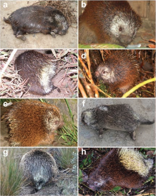
Figure 1 New records of Coendou rufescens in Ecuador: a = Road in the vicinity of Chaguarpamba, b = Quilanga, c = Olmedo, d = vicinity of the Villonaco Wind Project, e = Barrio Zamora Huayco, f = Vicinity of Gonzanama, G = Camino del Inca, and h = 5 km of Saraguro. a-f and h = province of Loja; h = province of Chimborazo.
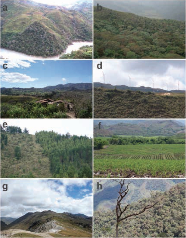
Figure 2 Localities of new records of Coendou rufescens in Ecuador: a = Road in the vicinity of Chaguarpamba, b = Quilanga, c = Olmedo, d = Vicinity of the Villonaco Wind Project, e = Barrio Zamora Huayco, f = Vicinity of Gonzanama, g = Camino del Inca, and h = 5 km of Saraguro. a-f and h = province of Loja; h = province of Chimborazo.
2) Quilanga, province of Loja: Individual kept as a pet, photographed (Figure 1b) on 23 June 2011. This specimen was captured in a forest with secondary vegetation adjacent to agricultural land (Figure 2b), montane cloud forest ecosystem, southern sector of the Western Cordillera, southern subregion (Valencia et al. 1999), Temperate zoogeographical area (Albuja et al. 2012).
3) Olmedo, province of Loja: Individual photographed (Figure 1c) on 18 February 2012. The area corresponds to an agricultural area (Figure 2c) located in a piedmont deciduous forest ecosystem, foothills of the Western Cordillera, southern subregion (Cerón et al. 1999), subtropical western zoogeographical area (Albuja et al. 2012).
4) Vicinity of the Villonaco Wind Project (Figure 1d), Sucre, province of Loja: Individual photographed on 17 March 2012. The site of the finding corresponds to a rural zone with secondary vegetation and agricultural fields (Figure 2d) pertaining to a mountain cloud forest, southern sector of the Western Cordillera, southern subregion (Valencia et al. 1999), western Andean high zoogeographical area (Albuja et al. 2012).
5) Zamora Huayco neighborhood in El Sagrario, province of Loja: The record corresponds to an individual (Figure 1e) photographed on 7 September 2012. This was observed in a planted conifer forest (Pinus sylvestris) adjacent to the boundary of the Podocarpus National Park (Figure 2e), montane cloud forest ecosystem, southern sector of the Western Cordillera, southern subregion (Valencia et al. 1999), Temperate zoogeographical area (Albuja et al. 2012).
6) Vicinity of the Gonzanamá, province of Loja: Roadkilled individual photographed on 28 September 2012 (Figure 1f). The area corresponds to an agricultural zone with small remnant patches of native vegetation (Figure 2f) pertaining to a mountain cloud forest, southern sector of the Western Cordillera, southern subregion (Valencia et al. 1999), Temperate zoogeographical area (Albuja et al. 2012).
7) Inner zone of the Sangay National Park, province of Morona Santiago: Individual (Figure 1g) photographed on 12 June 2015 in a high Andean moorland in the Camino del Inca sector (Figure 2g). Andean High zoogeographical area (Albuja et al. 2012).
8) 5 km from Saraguro, province of Loja: Specimen (Figure 1h) photographed on 17 June 2017 in the Huashapamba forest, in an area between shrub vegetation and a pasture located in the western part crossed by the Pan-American Highway. The area is located inside a protected natural forest (Figure 2h) pertaining to a mountain cloud forest, southern sector of the Western Cordillera, southern subregion (Valencia et al. 1999), Andean High zoogeographical area (Albuja et al. 2012).
9) El Tuni, province of Azuay: MEPN 10433.
10) San Francisco Scientific Station, province of Zamora Chinchipe: MEPN 3260.
The individuals observed and photographed displayed morphological traits consistent with the description for the species (Voss 2015), namely short, blackish, non-prehensile tail measuring about 40% of the head-body length. Chin, throat and abdomen of pale brown color.
Potential Distribution. An AUC of 0.969 (min = 0.945, max = 0.98, σ = 0.007, n = 50) and a AUC ratio of 1.89 ± 0.04 (P < 0.05) were obtained. Fourteen variables with a significant contribution to the model were identified (Table 1); however, variables BIO1, BIO3, BIO7, BIO8, BIO10, BIO11, BIO13, BIO16 and BIO17 were eliminated for being highly correlated (Figure 3). Five non-correlated bioclimatic variables made a significant contribution to the model; seasonal temperature (BIO4) and minimum temperature of the coldest month (BIO6) accounted for 82.7 %, whereas precipitation of the fourth warmer quarter (BIO18), precipitation of the fourth annual quarter (BIO19), and precipitation of the driest month (BIO14) contributed 17.3 %.
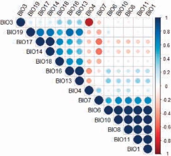
Figure 3 Correlation chart of the bioclimatic variables that make a significant contribution to the predictive model of the distribution of Coendou rufescens.
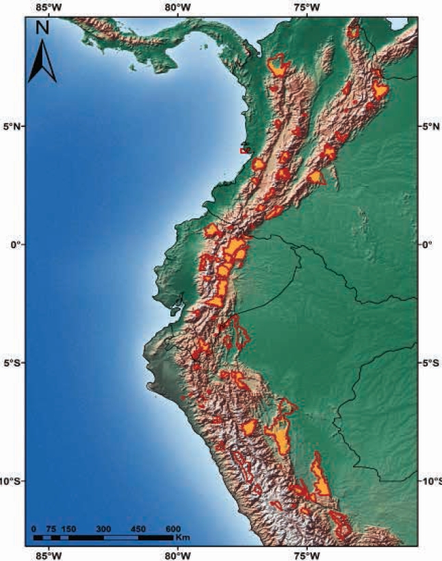
The area of suitable habitat predicted by the model for C. rufescens was ~448.820 km2, which in Colombia spans from the north end of the Eastern Cordillera, crossing the Central and Western Cordillera and Nudo de los Pastos; in Ecuador, this species is distributed in the Andean foothills and moorlands throughout the territory. In Peru, it stretches across the northern and central Andes in Western, Central and Eastern Cordilleras (Figure 4). Colombia has 50.4 % of the suitable distribution of the species, while Peru and Ecuador show 28.5 % and 21.1 %, respectively (Table 2). The potential distribution of C. rufescens in relation to remnant vegetation is reduced in 50.6 % (Table 2, Figure 4), with Peru and Colombia keeping 73 % (40.2 % vs 32.8 %) of remnant vegetation within the potential distribution range of the species (Figure 5). The potential distribution coinciding with the borders of protected areas in the three countries is 14 %, with Ecuador and Colombia keeping 10 % (Table 2, Figure 5).
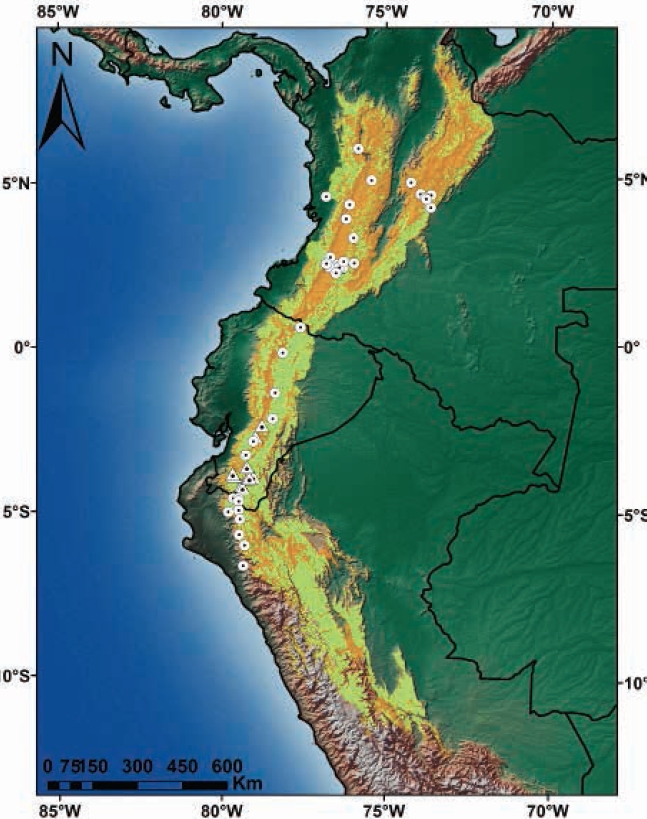
Figure 4 Records and potential distribution of Coendou rufescens (orange), potential range of C. rufescens in relation to remnant vegetation in Colombia, Ecuador and Peru (light green). Circles represent records from the literature review; triangles, the new locations reported in this study.
Table 2 Percentage of potential distribution and remnant vegetation of the predictive model for Coendou rufescens.
| Country | Potential Distribution km2 (%) | Remnant vegetation km2 (%) | Potential distribution within protected areas (%) |
|---|---|---|---|
| Colombia | 226,146 (50.4) | 72,675 (32.7) | 21,931 (34.9) |
| Peru | 128,104 (28.5) | 89,252 (40.2) | 18,522 (29.5) |
| Ecuador | 94,570 (21.1) | 59,665 (26.9) | 22,279 (35.5) |
| Total | 448,820 (100) | 221,592 (100) | 62,732 (100) |
Discussion
In Ecuador, the distribution range of C. rufescens was known by few and scattered records along the Eastern Cordillera, with a single record from the Western Cordillera (Orcés and Albuja 2004; Voss 2015; Vallejo and Boada 2017; Romero et al. 2018). The localities reported in this study broaden the distribution range of the species to the south and southwest areas of the Eastern and Western Cordillera across an altitudinal range of 1.120-4.387 m. The Camino del Inca locality in the Sangay National Park at 4,387 masl is the highest-elevation record for the species (Appendix 1) and for the family Erethizontidae (Voss 2015; Barthelmess 2016). High elevations are characterized by extreme weather conditions, where only the best-adapted species are able to thrive (Monge and León-Velarde 1991); thus, mammals that inhabit ecosystems above 4,300 m asl are currently scarce in Ecuador (< 10 spp.) (Tirira 2017; Brito et al. 2018).
Observations by the authors and references provided by local residents indicate that C. rufescens inhabiting southwest areas move at ground level and climb easily, being tolerant to anthropic areas such as villages and farming land; a similar behavior has been documented for Peruvian (More and Crespo 2016) and Ecuadorian populations (Brito and Ojala-Barbour 2016). Similar to other related species (Voss 2015), the specimens of C. rufescens observed in this study showed a quiet temperament and adopted a still position, hiding the head and ruffling up the spines when perceiving danger. In the province of Loja, local peasants frequently capture specimens of C. rufescens resting on tree branches to keep them as pets and/or for consumption as bush meat. Rhodas et al. (2007) report this as one of the species most commonly marketed in southern Ecuador.
The distribution of Coendou rufescens predicted by the model yielded a high AUC, and the AUC ratio in the analysis of partial ROC curves showed that the predictive capability of the model is significantly better than the one produced by a random model (Hanley and McNeil 1982; Lobo et al. 2008; Peterson et al. 2008) and may be a similar representation to the distribution range of the species. The results of this study are consistent with the distribution reported elsewhere (Alberico et al. 1999; Orcés and Albuja 2004; Voss 2011; Brito and Ojala-Barbour 2016; More and Crespo 2016; Romero et al. 2018), although the suitable habitat that may be occupied by the stump-tailed porcupine was maximized; thus, the maximum entropy principle allowed us to model the convergence of environmental variables (Phillips et al. 2006) in a total area of ~448.820 km2. However, our map — predictive model — does not display the actual geographical distribution of the species, as the existence of a suitable habitat is no guarantee that the species indeed inhabits the whole habitat. However, the absence of C. rufescens in an area of suitable habitat could be the result of biotic interactions (e. g. competition with other species, presence of predators) or the inability of the species to move across geographical barriers (e. g. rivers, canyons, mountains, etc.) to colonize that habitat.
It is considered that the two bioclimatic variables that made a significant contribution to the predictive distribution model of C. rufescens — seasonal temperature (BIO4) and minimum temperature of the coldest month (BIO6) — are associated to the habitat occupied by the species (Ministerio del Ambiente del Ecuador 2013; Voss 2015; Brito and Ojala-Barbour 2016; More and Crespo 2016). The relationship between the Andean mountain ranges and these variables is displayed in the case study for small vertebrates; Muñoz-Ortiz et al. (2015) report that the localities of Rheobates (Anura) at the Central Cordillera are related to seasonal temperature (BIO4), whereas the localities at the Eastern Cordillera relate to the minimum temperature of the coldest month (BIO6). Coendou rufescens are distributed along the Western, Central and Eastern Cordillera, which explains a > 80 % contribution by the two variables.
In a number of studies, the maximum entropy model (MaxEnt) has yielded a better performance vs. other species-distribution models (Elith et al. 2006; Phillips et al. 2006; Aguirre-Gutiérrez et al. 2013), and some studies support that the ability of the algorithm to model the predictive distribution of the species is superior to that of other algorithms; however, these authors suggest that consensus models may be used in order to reduce the uncertainty in the predictions of individual models (Marmion et al. 2009; Qiao et al. 2015; Zhu and Peterson 2017). However, irrespective of the model — or a consensus of models — used, caution should be exercised when extrapolating data from the model, as it will depend on the objectives of the research.
Although Colombia is the country with the greatest portion of the potential distribution of the stump-tailed porcupine, when evaluating the proportion related to remnant vegetation, Peru comprises 20 % of the remaining distribution with respect to this variable, being the country with greatest coverage for the species. For its part, Colombia shows highly fragmented habitats in the western, central and eastern foothills (SIAC 2017), similar to Ecuador, which also faces threats related to habitat fragmentation in the Andes (Ministerio del Ambiente del Ecuador 2013; Lozano et al. 2006). However, the presence of continuous protected areas in Ecuador — mostly in the eastern slope — may ensure the mid-to-long-term permanence of the species.
Finally, the fact that several of our records correspond to road killed individuals evidences the need to implement measures to reduce the impact of roads on natural populations of this and other wild species, such as the construction of structural crossing tunnels/bridges (at least in the vicinity of National Park), in addition to implementing adequate signaling (Bank et al. 2002; Grillo et al. 2010).

