SciELO - Scientific Electronic Library Online

 
vol.8 número2Habitat and abundance of the Neotropical otter (Lontra longicaudis annectens) in Pueblo Nuevo, Durango, MexicoRichness and trophic guilds of carnivorous mammals in ejido Nuevo Becal, Calakmul, Campeche, Mexico índice de autoresíndice de materiabúsqueda de artículos
Home Pagelista alfabética de revistas  

Servicios Personalizados

Revista

Articulo

Indicadores

Links relacionados

  • No hay artículos similaresSimilares en SciELO

Compartir


Therya

versión On-line ISSN 2007-3364

Therya vol.8 no.2 La Paz may. 2017

https://doi.org/10.12933/therya-17-478 

Articles

Estimating the potential distribution and conservation priorities of Chironectes minimus (Zimmermann, 1780) (Didelphimorphia: Didelphidae)

David A. Prieto-Torres1  2  3  * 

Gonzalo Pinilla-Buitrago2  4  5 

1 Eje BioCiencias, Centro de Modelado Científico de la Universidad del Zulia (CMC-LUZ), Facultad Experimental de Ciencias. Calle 65 con Av. Universidad, sector Grado de Oro, Estado Zulia, Maracaibo 4004, Venezuela. E-mail: dprieto@cmc.org.ve (DAPT)

2 Red de Biología Evolutiva, Laboratorio de Bioclimatología, Instituto de Ecología, A.C. Carretera antigua a Coatepec 351, CP. 91070, Xalapa. Veracruz, México. E-mail: gepinillab@gmail.com (GEPB)

3 Museo de Biología de la Universidad del Zulia (MBLUZ), Facultad Experimental de Ciencias. Calle 65 con Av. Universidad, sector Grado de Oro, Estado Zulia, Maracaibo 4004, Venezuela.

4 Grupo de Mastozoología Universidad Nacional de Colombia, Facultad de Ciencias, Universidad Nacional de Colombia. Calle 26, Bogotá 111321. Distrito Capital, Colombia.

5 Grupo en Conservación y Manejo de Vida Silvestre, Instituto de Ciencias Naturales, Facultad de Ciencias, Universidad Nacional de Colombia Calle 26, Bogotá 111321. Distrito Capital, Colombia.


Abstract:

The water opossum (Chironectes minimus) is an elusive and solitary Neotropical semi-aquatic species, whose population dynamics cannot be studied using traditional methods to capture small mammals. Therefore, some aspects of its distribution, habitat requirements, and abundance are mostly unknown; which makes a proper determination of its conservation status difficult. Considering that new techniques known as species distribution models (SDMs) allow us to estimate the suitable areas and the most important variables for the distribution of a species, we compiled water opossum occurrences and modeled its potential distribution on a continental scale. We performed a SDM for the water opossum using MaxEnt and assessed the extent of habitat loss (km2) and the importance of Protected Areas (PAs). We compared the suitability values within and outside PAs using a Kolmogorov-Smirnov (KS) test to evaluate the efficiency of PAs. The results obtained were compared with the IUCN historical water opossum’s map. Additionally, we identified gaps in the potential distribution where for future surveys should be focused. We obtained models that describe the distribution of this species based on 292 occurrences with new information for 16 countries. Deforestation reduced the area of suitable habitat by ~40 % and only ~18 % corresponds to natural forest within PAs. Areas inside PAs showed higher suitability values (0.351 ± 0.276; P < 0.001) than areas outside them. We identified gaps within the distribution that need attention during future surveys such as the frontier between Venezuela and Guyana, the Amazonian region, and central-eastern Brazil. Our results showed areas absent in the IUCN’s distribution map, indicating that it needs to be updated. Thus, we proposed a new tentative extent of the water opossum distribution information here obtained. We demonstrated that PAs included areas with high habitat suitability values for C. minimus, which could protect the water opossum in the medium and long-term. Modifications to the physicochemical characteristics of the habitat due to forest loss and fragmentation can considerably affect water opossum populations and reduce local diversity. Thus, the preservation of river ecosystems and surrounding areas represents a necessary step for the conservation of C. minimus.

Key words: conservation; ecological niche models; mammals; marsupials; species distribution models; water opossum

Resumen:

La zarigüeya de agua (Chironectes minimus) es una especie neotropical semi-acuática, de hábitos esquivos y solitarios, cuya dinámica poblacional no puede ser estudiada métodos tradicionales de captura de pequeños mamíferos. Es por ello que algunos aspectos de su distribución, sus requerimientos de hábitat y su abundancia siguen siendo desconocidos, dificultando su apropiada categorización. Considerando que modelos de distribución de especies (MDE) nos permiten estimar y las variables climáticas más importantes para la distribución; se recopilaron las ocurrencias de C. minimus y se modelo su distribución potencial a una escala continental. Utilizando el programa MaxEnt se definió un MDE para la zarigüeya de agua, evaluando el efecto de la pérdida de hábitat (km2) y la importancia de las Áreas Protegidas (AP) en la extensión del mismo. La eficiencia de las APs fue evaluada con una prueba de Kolmogorov-Smirnov (KS) para comparar los valores de idoneidad del MDE obtenidos dentro y fuera de las APs. Los resultados obtenidos se compararon con el mapa de distribución histórica de la UICN. Adicionalmente, se identificaron vacíos de información en la distribución potencial donde enfocar esfuerzos de muestreo mediante el cálculo de un índice de prioridad. Se obtuvieron modelos a partir de 292 ocurrencias, con nueva información en 16 países. La deforestación redujo la distribución potencial en ~ 40 % y se observó que solo el ~ 18% corresponde a bosques naturales dentro de las AP. Las áreas de distribución potencial mostraron valores de idoneidad más altos dentro de las APs (0,351 ± 0,276, p < 0,001). Las áreas con vacíos de información fueron identificadas en la frontera entre Venezuela y Guyana, la región amazónica y el centro-este de Brasil. Los resultados indican áreas de distribución ausentes en el mapa de la UICN, sugiriendo que este necesita ser actualizado. Por lo tanto, se propone una nueva distribución de la zarigüeya de agua. Se demostró que las APs incluyeron áreas con altos valores de idoneidad de hábitat para C. minimus; lo que podría favorecer su protección a medio y largo plazo. Las modificaciones de las características fisicoquímicas del hábitat por la pérdida y fragmentación de los bosques pueden afectar considerablemente a las poblaciones de zarigüeyas de agua y reducir la diversidad local. La preservación de los ecosistemas fluviales y las áreas circundantes en su conjunto representa un paso esencial para la conservación de C. minimus.

Introduction

The water opossum or Yapok, Chironectes minimus (Zimmerman 1780), is the only Neotropical semi-aquatic marsupial (Bressiani and Graipel 2008; Acosta and Azurduy 2009; Galliez et al. 2009). It belongs to a monotypic genus, which includes four subspecies (Stein and Patton 2007; Damasceno and Astúa 2016). The species is characterized by a silvery gray dorsal pelage with four black transverse patches connected by a narrow midline. Water opossums are adapted to semi-aquatic habitats, with several external morphological adaptations: 1) dense, short, and water-resistant pelage, 2) webbed hindfeet to swim, 3) impermeable pouch in females to keep the young dry, and 4) the ability to protect the male genitalia in the water with an incomplete pouch (Mondolfi and Medina 1957; Marshall 1978; Stein and Patton 2007; Voss and Jansa 2009).

Water opossums are widely distributed in the Neotropics (Figure 1), from southern Mexico to northeastern Argentina (Nowak 1999; Cuarón et al. 2008). This elusive and solitary species is mainly associated with river channels with stony substrates, clear and fast-running waters, and preserved riparian vegetation (Prieto-Torres et al. 2008; Galliez et al. 2009; Galliez and Fernandez 2012; Ardente et al. 2013). However, it is a species whose large-scale population dynamics (e. g., distribution and abundance) cannot be studied using traditional methods, because they are not usually captured in common live traps for small mammals (Bressiani and Graipel 2008; Prieto-Torres et al. 2011). In fact, although there are some studies on the behavior, demographic patterns, habitat selection, morpho-physiological and genetic analyses of water opossums (e. g., Nogueira et al. 2004; Galliez et al. 2009; Palmeirim et al. 2014; Fernandez et al. 2015), most of them are not-specific, faunistic surveys (e. g., Handley 1976; Oliveira et al. 2007; Prieto-Torres et al. 2008; 2011; Ardente et al. 2013).

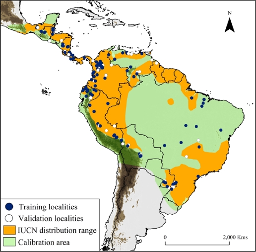
Figure 1 Map showing water opossum (Chironectes minimus) unique records (n = 165), overlaid with the IUCN distribution and model calibration area (light and dark green colors). Training localities (blue dots) and validation localities (white dots) were used to generate and validate the models. Dark brown color represents area with altitudes of up 1,200 m. 

The water opossum is listed as Least Concern (Cuarón et al. 2008) on the International Union for Conservation of Nature (IUCN) red list due to its wide distribution, presumably large population, and its presence in several protected areas or “PAs” (Oliveira et al. 2007; Galliez et al. 2009; Ardente et al. 2013). However, recent work suggests a decreasing population trend in Brazil, where the species is considered threatened in at least five states due to habitat loss and degradation (Ardente et al. 2013; Palmeirim et al. 2014; Fernandez et al. 2015). Thus, there is an increasing need to define its actual distribution and ecological requirements (Cuarón et al. 2008).

The minimum convex polygon method is frequently used to estimate species’ distribution (IUCN 2001, 2015), but ignores the species’ ecological constraints (Brown et al. 1996; Mota-Vargas and Rojas-Soto 2012; Peterson et al. 2016). Thus, techniques like species distribution models (SDMs) have been developed to predict the potential distribution of a species, identifying the suitable areas and the most important variables for the persistence of the species (Peterson 2001; Soberón and Peterson 2005; Stohlgren et al. 2011). These models are widely used in ecology, evolution, conservation, and management (e. g., Soberón and Peterson 2005; Stohlgren et al. 2011; Tôrres et al. 2012; Ortega-Andrade et al. 2013; 2015).

Due to the lack of information on the distribution of C. minimus, in this study we modeled its potential distribution on a continental scale, following part of the methodology of Rheingantz et al. (2014) employed for another semi-aquatic mammal. We determined the effect of habitat loss in the extents of habitat suitability for species and evaluated if the current PAs systems actually harbor the most suitable environmental conditions for its distribution. Finally, we identified gaps in the potential distribution where future survey efforts and ecological studies should be focused.

Material and Methods

Collection of historical records. We compiled a database of occurrences from three sources: 1) occurrences available in on-line databases (i. e., Global Biodiversity Information Facility database [GBIF] and Mammal Networked Information System [MaNIS]); 2) specimens verified from biological collections (see Appendix 1); and 3) location records obtained from fieldwork and published literature (e. g., Handley 1976; Mares et al. 1986; Oliveira et al. 2007; Bressiani and Graipel 2008; Prieto-Torres et al. 2008; 2011; Acosta and Azurduy 2009; Ardente et al. 2013; Brandão et al. 2014; Damasceno and Astúa 2016). We verified each locality using Google Earth and MapLink (http://www.maplink.com), correcting imprecise coordinates and/or eliminating duplicates when necessary. Geographic coordinates were provided in decimal degrees, based on the WGS 84 datum. We obtained data from sixteen countries between 1925 and 2015 describing the historical presence of the species (Figure 1, Appendix 1). In addition, we considered the largest water opossum home range (~3 km2; Galliez et al. 2009) as a buffer area between records and cleared the points located close together, thereby reducing sampling bias (e. g., Ortega-Andrade et al. 2015). We performed the SDM (see below) using 165 unique localities records (Appendix 1).

Species Distribution Model and validation. We modeled the potential water opossum distribution with MaxEnt version 3.3.3k (Peterson 2001; Elith et al. 2006; Phillips et al. 2006), which uses the principle of maximum entropy to calculate the most likely distribution of the focal species in function of occurrence localities and environmental variables. We used the 19 climatic variables of WorldClim 1.4 (Hijmans et al. 2005) and three topographic variables (i. e., Digital Elevation Model [DEM], Slope and Aspect) from the Hydro 1K project (USGS 2001); with 30” of resolution (~1 km2 cell size). Despite that topographic variables are not commonly used in SDM studies, they were included because numerous examples (e. g., Mota-Vargas et al. 2013; Cauwer et al. 2014; Rheingantz et al. 2014; Kübler et al. 2016) show that these variables can be used as proxies for variables (e. g., micro-climate or edaphic conditions) that are correlated with physiological requirements of species.

The potential distribution model was generated using the 75 % (n = 124) of the locality records and 25 % (n = 41) for internal evaluation. In this sense, the algorithm used localities of species records and environmental conditions to perform a certain number of iterations (1,000 in this case) before reaching a convergence limit. This algorithm for the logistic output produces a map of habitat suitability ranging from 0 (unsuitable) to 1 (perfectly adequate; Phillips et al. 2006; Phillips and Dubik 2008). We ran ten cross-validate replicates to calculate confidence intervals, and the best model was selected based on the performance of area under the curve or “AUC” (Elith et al. 2006; 2011). Then, we converted the obtained logistic values of suitability rating into a binary presence-absence map, based on two established threshold values: the “Fixed cumulative value 10” (FCV10) and the “5 percentile training presence” (5PTP; see Pearson et al. 2006; Liu et al. 2013).

It is important to note that there is no rule to set these thresholds because its selection depends on the data used or the objective of the map, and will vary from species to species. In our case, we used the FCV10 as we wanted a threshold that minimizes the commission errors in our final binary maps (Liu et al. 2013), and we used the 5PTP to identify pixels with the highest suitability values, rejecting the lowest (5 %) suitability values of training records. The 5PTP model is a sub-conjunct in the geographic and ecological space of FCV10 model.

Given that ENMs do not address the historical aspects relating to species distribution (e. g., accessibility or “M” sensu BAM diagram [Soberón and Peterson 2005]), we used a geographical clip (Figure 1; Appendix 2) based on the intersection of Terrestrial Ecoregions (Olson et al. 2001) and the Biogeographical Provinces of the Neotropic (Morrone 2014) to create an area for model calibration (see Anderson and Raza 2010; Barve et al. 2011; Rodda et al. 2011). We selected the uncorrelated (r < 0.8) and most relevant variables using the Jackknife test of MaxEnt (Royle et al. 2012). These steps allowed us to reduce over-fitting of the generated suitability models (Peterson et al. 2011). Finally, we evaluated the performance of the selected MaxEnt model with the Partial-ROC (Receiver Operating Characteristic) curves test (Lobo et al. 2008). This criterion was used to solve problems associated with an inappropriate weighting of the omission and commission errors during the AUC analysis (see Lobo et al. 2008; Peterson et al. 2008).

Spatial analysis of the water opossum’ distribution in the Neotropics. We performed three distinct spatial analyses to assess the conservation issues related to the species’ potential distribution: 1) to evaluate the extent of habitat loss on the model; 2) to determine if the PAs system contains the highly suitable areas for the species; and 3) to identify the gaps where future survey efforts should be focused. The spatial analyses and map algebra were carried out with ArcMap 10.2.2 software (ESRI 2011), with a grid cell resolution of 30’’, corresponding to ~1 km2 in each raster.

First, we used a vegetation land cover map (Hansen et al. 2013) considering only two categories “natural forest” and “perturbed areas,” to determine the effect of habitat loss in the obtained models. Perturbed areas included urban areas, deforested areas, farm lands, and pastures for cattle ranching (Hansen et al. 2013). The PAs extents were downloaded from ProtectedPlanet.net (IUCN and UNEP-WCMC 2012). To assess if the current PA system harbors the most suitable environmental conditions for the species we performed a Kolmogorov-Smirnov (KS) test in R (R-Core-Team 2012) comparing the suitability values within and outside PAs (Rheingantz et al. 2014). The results obtained from the deforestation and PAs analysis were compared with the IUCN species distribution.

Finally, to identify gaps in the potential distribution where future survey efforts and conservation initiatives should be focused, we followed the proposal by Rheingantz et al. (2014). In the analysis, we multiplied the suitability value of a pixel by its distance to the nearest occurrence and river, based on the assumption that ecological similarities decrease with distance among these factors. Then, we divided the index by its highest value to obtain a scale from 0 to 1. We therefore assumed that areas with high suitability values, located far from previous studies and near to rivers (the focal species is associated with water) were more likely to be in different ecosystems or to have dissimilar environmental characteristics (Rheingantz et al. 2014). Thus, studying water opossum in those areas could explain whether the species uses different habitats than previously reported.

Results

Historical records and SDM for water opossum. Our study includes new information on the distribution of water opossum, including a total of 292 occurrences in the 16 countries that encompass the recognized distribution ranges according to the IUCN (Figure 1; Marshall 1978; Cuarón et al. 2008). Including also new potential areas of distribution in Mexico, El Salvador, Nicaragua, Costa Rica, Colombia, Venezuela, Brazil, Bolivia, Peru and Ecuador.

The variables used and their percentage contribution to the model are shown in the Table 1 and are consistent with results found by previous studies on Neotropical mammals (e. g., DeMatteo and Loiselle 2008; Tôrres et al. 2012; Rheingantz et al. 2014). We generated a model for water opossum distribution with a high Roc-Partial result (1.23 ± 0.09; P < 0.05). For the threshold FCV10 (0.160) and 5PTP (0.190), based on 41 test occurrences, we obtained 7 % (n = 3) and 5 % (n = 2) rates of omission, respectively. Performance assessment showed that models were statistically acceptable to describe the ecological niche and distribution of this species.

Table 1 Summary of the selected environmental variables with relative contributions (%) to the model of Chironectes minimus using MaxEnt 3.3.3k 

Abbreviation Environmental Variable Percentage contribution
Bio 18 Precipitation of Warmest Quarter 24.7
Bio 11 Mean Temperature of Coldest Quarter 17.2
DEM Digital Elevation Model 16.5
Bio 07 Temperature Annual Range (BIO5-BIO6) 13.1
Bio 14 Precipitation of Driest Month 12.9
Bio 04 Temperature Seasonality (standard deviation *100) 7.8
Bio 15 Precipitation Seasonality (Coefficient of Variation) 5.4
Bio 01 Annual Mean Temperature 1.4
Bio 03 Isothermality (BIO2/BIO7) (* 100) 0.9

The water opossum potential distribution according to the FCV10 threshold totaled ~9,238,000 km2, representing 45.9 % of the total areas used in the calibration of the model (Figure 2a). This FCV10 model is ~23 % wider than IUCN’s historical distribution map (with ~72.29 % overlap). Considering the 5PTP threshold, we obtained ~7,787,700 km2 of potential distribution for the species, representing 38.3 % of calibration areas and is ~4 % greater than the IUCN’s distribution map (with ~65 % overlap). The 5PTP’s potential species distribution was smaller in almost all countries compared to the IUCN map (Figure 2a). Comparing the IUCN map and FCV10 threshold, the only regions absent in the latter were predominantly areas in Mexico, savanna in Colombia and Venezuela, amazon in Peru, and the southeast of Brazil.

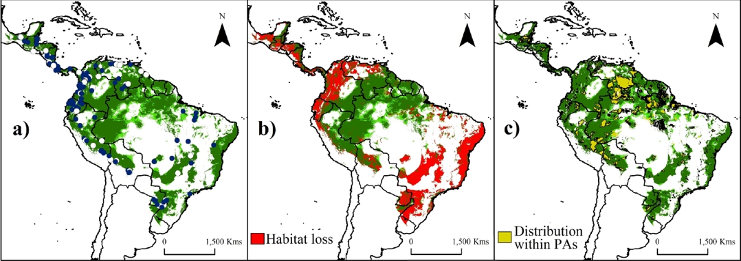
Figure 2 Potential suitability areas (a), remnant of natural forests (b) and predicted Protected Areas (c) throughout the distribution range of water opossum (Chironectes minimus). Training localities (blue dots) and validation localities (white dots) used to generate models are shown in (a). Potential distribution model (in a-c) is shown with the threshold value of Fixed cumulative value 10 (FCV10, light green) and 5 Percentile training presence (5PTP; dark green). Note an important reduction (~40 %, in greens [natural forests areas]) in the potential distribution model through the Mesoamerican region (from Mexico to Panama), the lowlands of the Andes region (from Peru to Colombia and northwest Venezuela), and the southeast of South America (Paraguay, Argentina and Brazil). The perturbed areas were calculated according the deforestation index map proposed by Hansen et al. (2013). Dark brown color represents area with altitudes of up 1,200 m. 

Deforestation impact, protected areas and future areas of study. The predicted and remnant areas of the potential distribution model for the water opossum according the threshold values are detailed in Tables 2 and 3. Deforestation reduced the area of suitable water opossum habitat by ~40 % (38.07 – 43.39 %). Loss in area was most pronounced in the Mesoamerican region (from Mexico to Panama), the lowlands of the Andes region (from Peru to Colombia and northwest Venezuela), and the southeast region of South America (Paraguay, Argentina and Brazil; Figure 2b). Furthermore, only ~18 % of the potential water opossum distribution corresponds to natural forest within PAs (Figure 2b-c; Tables 2-3).

Table 2 Potential distribution models for Chironectes minimus, with percentage loss of potential distribution areas by effect of habitat loss and the percentage of potential distribution within Protected Areas (PAs) in the Neotropics 

Model Area (~km2) %
Extent of occurrence (minimum convex polygon) 13,878,685 -
IUCN distribution map 7,501,124 100.00
Area of the model within natural forests 4,246,209 56.61
Area of the model within PAs 1,126,857 15.02
Remnant model within PAs and natural forests 978,935 13.05
Species Distribution Model (FCV10) 9,238,072 100.00
Area of the model within natural forests 5,721,975 61.93
Area of the model within PAs 1,840,152 19.91
Remnant model within PAs and natural forests 1,644,964 17.81
Species Distribution Model (5PTP) 7,787,759 100.00
Area of the model within natural forests 4,726,649 60.69
Area of the model within PAs 1,547,148 19.87
Remnant model within PAs and natural forests 1,381,237 17.74

Table 3 Potential distribution of water opossum (Chironectes minimus) estimated by country. Potential distributions are in km2 and percentages for each country, considering the deforestation effects and PAs, based in the two threshold values used in this study. 

Country FCV10 5PTP
Modeled Area (%) Intact Areas (%) Intact areas in PAs (%) Modeled Area (%) Intact Areas (%) Intact areas in PAs (%)
Brazil 4,555,022 (49.31) 2,642,873 (28.61) 774,870 (8.39) 3,604,227 (46.28) 1,980,563 (25.43) 569,951 (7.32)
Colombia 1,042,751 (11.28) 569,586 (6.16) 58,024 (0.63) 953,324 (12.24) 523,079 (6.72) 56,206 (0.72)
Venezuela 831,292 (8.99) 590,105 (6.38) 383,794 (4.15) 741,999 (9.53) 549,763 (7.06) 366,851 (4.71)
Peru 744,347 (8.06) 653,448 (7.07) 136,241 (1.47) 651,262 (8.36) 567,470 (7.28) 124,656 (1.60)
Bolivia 383,783 (4.15) 270,766 (2.93) 77,297 (0.84) 321,390 (4.12) 220,288 (2.83) 66,861 (0.86)
Ecuador 248,756 (2.69) 117,683 (1.27) 31,479 (0.34) 239,138 (3.07) 113,795 (1.46) 30,714 (0.39)
Guyana 211,967(2.29) 201,563 (2.18) 19,638 (0.21) 172,955 (2.22) 163,320 (2.09) 17,797 (0.23)
Mexico 206,711 (2.24) 91,310 (0.98) 20,817 (0.22) 183,380 (2.35) 83,238 (1.06) 17,907 (0.23)
Suriname 155,010 (1.68) 150,754 (1.63) 16,497 (0.18) 126,002 (1.62) 122,293 (1.57) 10,965 (0.14)
Paraguay 154,595 (1.67) 41,180 (0.44) 2,809 (0.03) 140,937 (1.81) 36,895 (0.47) 2,803 (0.04)
Nicaragua 114,767 (1.24) 64,038 (0.69) 12,556 (0.14) 112,145 (1.44) 63,173 (0.81) 12,546 (0.16)
Honduras 112,529 (1.22) 44,931 (0.48) 6,798 (0.07) 108,749 (1.39) 44,418 (0.57) 6,650 (0.08)
Guatemala 108,169 (1.17) 53,141 (0.57) 22,504 (0.24) 103,319 (1.33) 50,843 (0.65) 21,417 (0.27)
Argentina 102,436 (1.11) 65,902 (0.71) 17,084 (0.18) 90,662 (1.16) 58,660 (0.75) 16,630 (0.21)
French Guiana 79,829 (0.86) 79,018 (0.85) 38,863 (0.42) 67,426 (0.86) 66,917 (0.86) 33,904 (0.43)
Panama 73,839 (0.79) 38,500 (0.41) 8,544 (0.09) 67,499 (0.87) 36,004 (0.46) 8,284 (0.11)
Costa Rica 49,732 (0.54) 23,037 (0.25) 8,452 (0.09) 47,761 (0.61) 22,519 (0.29) 8,398 (0.11)
Uruguay 30,447 (0.33) 1,642 (0.017) 207 (0.002) 24,400 (0.31) 1,063 (0.013) 207 (0.002)
Belize 24,201 (0.26) 19,666 (0.21) 8,248 (0.09) 24,200 (0.31) 19,666 (0.25) 8,248 (0.11)
Trinidad and Tobago 4,909 (0.05) 2,402 (0.02) 228 (0.002) 4,785 (0.06) 2,385 (0.03) 228 (0.003)
El Salvador 2,980 (0.03) 430 (0.004) 14 (0.0001) 2,199 (0.03) 297 (0.003) 14 (0.0002)
Total 9,238,072 (100) 5,721,975 (61.93) 1,644,964 (17.81) 7,787,759 (100) 4,726,649 (60.69) 1,381,237 (17.74)

The current PAs system in the Neotropics represents ~20 % of species’ potential distribution (Figure 2c). Areas inside PAs showed significantly higher suitability values (0.351 ± 0.276; KS, P < 0.001) than areas outside them (0.319 ± 0.238). The highest values were obtained in the Amazon areas (including Bolivia, Peru, Ecuador, Colombia, Venezuela, and Brazil; Figure 2), followed by the Guiana shield and the coast of the Atlantic forest. The index of suitable value multiplied by its distance to nearest occurrence and river identified gaps (index > 0.5) within the distribution that need attention during future surveys, such as the frontier between Venezuela and Guyana (mainly in the Guiana Highlands), the Amazonian region (including Colombia and the northwestern Brazil), and central-eastern Brazil (Figure 3a).

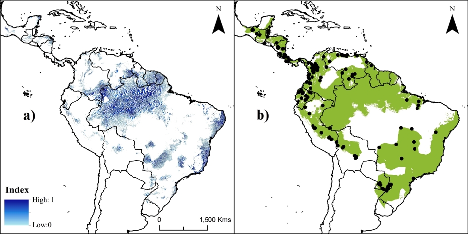
Figure 3 Maps showing priority areas for future studies (a) and the current proposed Neotropical distribution for water opossum, Chironectes minimus (b). Color palette in A corresponds to areas defined as priorities (from zero [light blue] to 1 [dark blue]) for future ecological studies and surveys for water opossum based on suitable value multiplied by its distance to nearest occurrence and water source (i. e., rivers). Black points in B represent the unique historical records (n = 165) of species. 

Discussion

Potential distribution range of water opossum and habitat loss effects. Our results confirm that the climate variables used in this study (Table 1) can be employed to model the potential distribution of terrestrial species associated with aquatic environments, as previously demonstrated for the otters Lontra longicaudis and Pteronura brasiliensis (Cianfrani et al. 2011; Rheingantz et al. 2014). Mean precipitation of the driest quarter and the warmest quarter were the most important variables for the water opossum’s distribution in the Neotropics (Table 1), as was found for the Neotropical otter (Rheingantz et al. 2014). Altitude was another important variable which represents a gradient correlating directly with factors such as micro-climate or edaphic conditions (Mota-Vargas et al. 2013; Kübler et al. 2016). Although water opossum occurred between zero to ~3,000 m (including the Andes region), most of the occurrences were between zero to 500 m (n = 81) and zero to 2,000 m (n = 157; Appendix 1). This spatial distribution of species’ occurrences suggests that the species has an altitudinal limit (due to climatic gradients by elevation) possibly associated with their physiological requirements. This last idea agrees with studies for the Neotropical otter, which is described as abundant at medium elevations (Lariviére 1999; Rheingantz et al. 2014).

It is important to observe that suitability model predicted for C. minimus was severely reduced due to habitat loss (~36 to 43 %); even inside of PAs (Tables 2 and 3). The habitat loss is associated with areas highly threatened by human activities (e. g., expansion of cattle ranching and urban settlements), which remove vegetation cover thereby reducing water opossum’s habitat (Prieto-Torres et al. 2008; 2011; Galliez et al. 2009). Similarly, previous studies report that the expansion of the agricultural frontier is a critical factor affecting biodiversity in the Neotropics (Shukla et al. 1990; Lees and Peres 2006; Bressiani and Graipel 2008; Ribeiro et al. 2009; Ortega-Andrade et al. 2015; Prieto-Torres et al. 2016). These conditions push the species to the edge of its distribution and increase fragmentation of predicted suitable areas, which could promote decreasing trends in populations (Ardente et al. 2013; Palmeirim et al. 2014; Fernandez et al. 2015). Thus, future conservation efforts should concentrate on reducing habitat loss and restoring identified natural habitats, especially considering the restricted home range and unknown population size of the water opossum (Galliez et al. 2009; IUCN 2015).

Protected areas and gaps in areas for future studies. We demonstrated that PAs included areas with high habitat suitability values for C. minimus, which could protect it in the medium and long-term. Furthermore, our analysis supports the idea that SDMs can be used to evaluate whether PAs are really conserving species within them. Such studies allow us to identify potential areas of conservation priority for the species to achieve more realistic conservation goals in their present and future distributions (e. g., Hannah et al. 2005, 2007; Dudley and Parish 2006; Lessmann et al. 2014).

The PAs system is especially important for the water opossum in the Amazon region, due to the low rate of deforestation of the remaining forest (Numata and Cochrane 2012). The persistence of PAs in this region will play a role in preventing environmental degradation in the central and south portion of the C. minimus. Meanwhile, populations along the Mesoamerican region (from Mexico to Panama), the western Andes (Ecuador, Colombia and Venezuela), and southeastern Brazil are more vulnerable to the effects of forest loss due to fewer PAs (Figure 2b-c). However, it is important to conserve not only PAs but also surrounding areas through forest restoration and sustainable development programs which include local people (Laurance et al. 2012; Rheingantz et al. 2014; Prieto-Torres et al. 2016). Additionally, studies under future climate change scenarios are needed to consider the role of the PAs system in protecting the species’ habitat (e. g., Hannah et al. 2005, 2007).

We suggest that future studies (e. g., inventories, population monitoring, abundance patterns, and habitat evaluations) need to be focused on the Guiana Highlands, the Amazonian region (including Colombia and northwestern Brazil), and central-eastern Brazil (Figure 3a). Working in unexplored areas frequently provides new information on a species in the form of expansion of known distribution ranges and new records of unidentified specimens (Soberón and Peterson 2005; Mota-Vargas and Rojas-Soto 2012; Tôrres et al. 2012; Ortega-Andrade et al. 2013; Rheingantz et al. 2014). Thus, our results aid in identifying unexplored areas where future survey efforts should be focused in order to accelerate the discovery of new populations of water opossum.

Implications for C. minimus’ conservation. Our results showed areas absent from the IUCN’s distribution map, indicating that this needs to be updated. Thus, we proposed a new tentative extent of the water opossum distribution (Figure 3b) which integrated the information obtained in the SDMs, the IUCN historical range, and the newly reported localities. This proposal includes new distribution areas for Mexico, Venezuela, Suriname, Guyana, Ecuador, Peru, Bolivia, and Argentina-Brazil; and at the same time reduces or eliminates areas in northern Brazil and the savanna in Colombia and Venezuela.

Clearly, the limited knowledge about the habitat requirements, distribution range, and information obtained directly from field activities, could explain why the water opossum is currently listed as Least Concern. At the continental level, there are mammals which have been reassigned because threat categories have been based more on anecdotal criteria than on field surveys and population assessments (e. g., Rheingantz and Trinca 2015). Apart from the problems associated with the lack of data for its categorization (Cuarón et al. 2008), our results in combination with the time elapsed since the first assignment justifies the need for a reassessment of the category, such as was done for L. longicaudis, whose threat category was up-listed from “Least Concern” to “Near Threatened” (Rheingantz and Trinca 2015).

On the other hand, it is important to note that our models showed that there is a disjunction in the distribution of water opossum, observed in the population of southeastern of Brazil (C. m. paraguanensis [Marshall 1978; Damasceno and Astúa 2016]). This disjunct distribution could represent ecological niche differences among subspecies, which could simultaneously affect the performance of our models (see Rojas-Soto et al. 2008; 2009; Mota-Vargas and Rojas-Soto 2016). It is reasonable to suggest that there are climatic and geographic factors acting (or that acted) as geographic barriers that contribute to the isolation of some populations (see Damasceno and Astúa 2016). Similar cases were documented for wide-ranging Didelphidae species: the genus Didelphis, the Black-eared opossums (D. marsupialis; Cerqueira 1985) and White-eared opossums (D. albiventris; Cerqueira and Lemos 2000), and the Lutrine Opossum, Lutreolina crassicaudata (Martínez-Lanfranco et al. 2014). From this perspective, our study suggests that the current taxonomic status of these populations needs to be adequately assessed using tools that could reveal their distinctiveness (Damasceno and Astúa 2016). Independently of the current taxonomic classification, a possible loss of one of these disjunct groups would be irreversible.

Although we only examined the environmental distribution of C. minimus, our results forecast a rapid decline in the potential distribution, principally attributed to a decrease in occupancy in areas affected by habitat loss and fragmentation (e. g. Prieto-Torres et al. 2011; Ardente et al. 2013; IUCN 2015; Palmeirim et al. 2014; Fernandez et al. 2015). Modifications to the physicochemical characteristics (e. g., water conditions) of the habitat due to the aforementioned processes can considerably affect water opossum populations and reduce local diversity, as found for other aquatic mammals (e.g., Bowyer et al. 1995; Rheingantz et al. 2014). Thus, considering physicochemical water conditions, the habitat structures to persist, and the habitat requirements to establish a viable population, will be crucial for the conservation of C. minimus and the preservation of river ecosystems as a whole.

Acknowledgements

We would like to acknowledge the contributions of the following organizations and individuals. Financial and logistical support was provided by Consejo de Desarrollo Científico, Humanístico y Tecnológico of Universidad del Zulia (CONDES) by the project CONDES CC-0247-13 (DAP-T). Authors extend their gratitude to Consejo Nacional de Ciencia y Tecnología (CONACyT, Mexico) for their postgraduate scholarships (297538 [DAP-T] and 395473 [GPB]). Museums that kindly providing data include: Estación Biológica Rancho Grande (EBRG) and Museo de Historia Natural La Salle (MHNLS) in Venezuela; Grupo de Mastozoología de la Universidad de Antioquia (GMUA) and Colección de Mamíferos “Alberto Cadena García” at Instituto de Ciencias Naturales (ICN), in Colombia; Museo Ecuatoriano de Ciencias Naturales (MECN) and Museo de Zoología de la Pontificia Universidad Católica del Ecuador (QCAZ-PUCE), in Ecuador; the Museo de Historia Natural de la Universidad San Agustín de Arequipa (MUSA), Peru; and the Museo de Historia Natural de Bolivia (MHNB), Bolivia. This manuscript was improved by comments from S. Solari, M. Delgado, F. J. García, and two anonymous reviewers. D. Spaan kindly reviewed the translation.

References

Acosta, L. S., and F. H., Azurduy. 2009. Nuevos Registros y apuntes sobre la carachupa de agua Chironectes minimus, en Los Valles Cruceños (Bolivia). Kempffiana 5:83-89. [ Links ]

Anderson, R. P., and A., Raza. 2010. The effect of the extent of the study region on GIS models of species geographic distributions and estimates of niche evolution: preliminary tests with montane rodents (genus Nephelomys) in Venezuela. Journal of Biogeography 37:1378-1393. [ Links ]

Ardente, N., D., Gettinger, R., Fonseca, H., de Godoy Bergallo H., and F., Martins-Hatano. 2013. Mammalia, Didelphimorphia, Didelphidae, Glironia venusta Thomas, 1912 and Chironectes minimus (Zimmermann, 1780): Distribution extension for eastern Amazonia. Check List 9:1104-1007. [ Links ]

Barve, N., V., Barve, A., Jiménez-Valverde, A., Lira-Noriega, S. P., Maher, A. T., Peterson, J., Soberón, and F., Villalobos. 2011. The crucial role of the accessible area in ecological niche modeling and species distribution modeling. Ecological Modelling 222:1810-1819. [ Links ]

Bowyer, R. T., J. W., Testa, and J. B., Faro. 1995. Habitat selection and home ranges of river otters in a marine environment: effects of the Exxon Valdez oil spill. Journal of Mammalogy 76:1-11. [ Links ]

Brandão, M. V., G. S., Terra Garbino, L., Perez Godoy, L., Alves da Silva, and W., Pascoal. 2014. New records of Chironectes minimus (Zimmermann, 1780) (Didelphimorphia, Didelphidae) from central Brazil, with comments on its distribution pattern. Mammalia 79:363-368. [ Links ]

Bressiani, V. B., and M. E., Graipel. 2008. Comparação de métodos para captura da cuíca-d’água, Chironectes minimus (Zimmermann, 1780) (Mammalia, Didelphidae) no sul do Brasil. Mastozoología Neotropical 15:33-39. [ Links ]

Brown, J. H., G. C., Stevens, and D. M., Kaufman. 1996. The geographic range: size, shape, boundaries, and internal structure. Annual Review of Ecology and Systematics 27:597-623. [ Links ]

Cauwer, V. D., B., Muys, R., Revermann, and A., Trabucco. 2014. Potential, realised, future distribution and environmental suitability for Pterocarpus angolensis DC in southern Africa. Forest Ecology and Management 315:211-226. [ Links ]

Cerqueira, R.. 1985. The distribution of Didelphis in South America (Polyprotodontia, Didelphidae). Journal of Biogeography 12:135-145. [ Links ]

Cerqueira, R., and B., Lemos. 2000. Morphometric differentiation between Neotropical black-eared opossums, Didelphis marsupialis and D. aurita (Didelphimorphia, Didelphidae). Mammalia 64:319-327. [ Links ]

Cianfrani, C., G., Le Lay, L., Maiorano, H. F., Satizábal, A., Loy, and A., Guisan. 2011. Adapting global conservation strategies to climate change at the European scale: The otter as a flagship species. Biological Conservation 144:2068-2080. [ Links ]

Cuarón, A. D., L., Emmons, K., Helgen, F., Reid, D., Lew, B., Patterson, C., Delgado, and S., Solari. 2008. Chironectes minimus. The IUCN Red List of Threatened Species. http://dx.doi.org/10.2305/IUCN.UK.2008.RLTS.T4671A11076156.en. Accessed 16.06.2016. [ Links ]

Damasceno, E. M., and D., Astúa. 2016. Geographic variation in cranial morphology of the Water Opossum Chironectes minimus (Didelphimorphia, Didelphidae). Mammalian Biology 81:380-392. [ Links ]

DeMatteo, K. E., and B. A., Loiselle. 2008. New data on the status and distribution of the bush dog (Speothos venaticus): Evaluating its quality of protection and directing research efforts. Biological Conservation 141:2494-2505. [ Links ]

Dudley, N., and J., Parish. 2006. Closing the Gap: Creating ecologically representative protected area systems. Technical Series No. 24. Montreal, QC: Secretariat of the Convention on Biological Diversity, Montreal. U. S. A. [ Links ]

Elith, J., C. H., Graham, R. P., Anderson, M., Dudík, S., Ferrier, A., Guisan, R. J., Hijmans, F., Huettmann, J. R., Leathwick, A., Lehmann, J., Li, L. G., Lohmann, B. A., Loiselle, G., Manion, C., Moritz, M., Nakamura, Y., Nakazawa, J. M., Overton, A. T., Peterson, S. J., Phillips, K. S., Richardson, R., Scachetti Pereira, R. E., Schapire, J., Soberón, S., Williams, M. S., Wisz, and N. E., Zimmermann. 2006. Novel methods improve prediction of species’ distributions from occurrence data. Ecography 29:129-151. [ Links ]

Elith, J., S. J., Phillips, T., Hastie, M., Dudík, Y. E., Chee, and C. J., Yates. 2011. A statistical explanation of MaxEnt for ecologists. Diversity and Distributions 17:43-57. [ Links ]

ESRI (Environmental Systems Research Institute). 2011. ArcGIS Desktop: Release 10, Environmental Systems Research Institute. Redlands, U. S. A. [ Links ]

Fernandez, F. A. S., M., Galliez, M. D. S., Leite, T. L., Queiroz, and A. F., Palmerim. 2015. Natural history of the water opossum Chironectes minimus: a review. Oecologia Australis 19:47-62. [ Links ]

Galliez, M., and F. A. S, Fernandez. 2012. Spatial segregation between the water opossum Chironectes minimus and the water rat Nectomys squamipes: just competition avoidance or a conservation problem as well? Mammalian Biology 77:447-450. [ Links ]

Galliez, M., M., de Souza Leite, T. L., Queiroz, and F. A. S., Fernandez. 2009. Ecology of the Water Opossum Chironectes minimus in Atlantic Forest Streams of Southeastern Brazil. Journal of Mammalogy 90:93-103. [ Links ]

Hannah, L., G. F., Midgley, G., Hughes, and B., Bomhard. 2005. The view from the Cape: extinction risk, protected areas and climate change. BioScience 55:231-42. [ Links ]

Hannah, L, G., Midgley, S., Andelman, M., Araújo, G., Hughes, E., Martinez-Meyer, R., Pearson, and P., Williams. 2007. Protected Area Needs in a Changing Climate. Frontiers in Ecology and the Environment 5:131-138 [ Links ]

Handley, C. O. Jr.. 1976. Mammals of the Smithsonian Venezuelan Project. Brigham Young University Science Bulletin - Biological Series 20:1-91. [ Links ]

Hansen, M. C., P. V., Potapov, R., Moore, M., Hancher, S. A., Turubanova, A., Tyukavina, D., Thau, S. V., Stehman, S. J., Goetz, T. R., Loveland, A., Kommareddy, A., Egorov, L., Chini, C. O., Justice, and J. R. G., Townshend. 2013. High-Resolution Global Maps of 21st-Century Forest Cover Change. Science 342:850-53. [ Links ]

Hijmans, R. J., S. E., Cameron, J. L., Parra, P. G., Jones, and A., Jarvis. 2005. Very high resolution interpolated climate surfaces for global land areas. International Journal of Climatology 25:1965-1978. [ Links ]

IUCN. 2001. Categorías y criterios de la Lista Roja de la UICN, Version 3.1. Comisión de Supervivencia de Especies de la UICN. UICN, Gland, Suiza y Cambridge, Reino Unido. [ Links ]

IUCN. 2015. The IUCN Red List of Threatened Species. Version 2015-4. http://www.iucnredlist.org Accessed 14.03.2016. [ Links ]

IUCN, and UNEP-WCMC.. 2012. Protected Planet - The latest initiative harnessing the World Database on Protected Areas. http://www.protectedplanet.net/ Accessed 09.02.2016. [ Links ]

Kübler, D., P., Hildebrandt, S., Günter, B., Stimm, M., Weber, R., Mosandl, J., Muñoz, O., Cabrera, N., Aguirre, J., Zeilinger, and B., Silva. 2016. Assessing the importance of topographic variables for the spatial distribution of tree species in a tropical mountain forest. Erdkunde 70:19-47. [ Links ]

Lariviére, S.. 1999. Lontra longicaudis. Mammalian Species 609:1-5. [ Links ]

Laurance, W. F., D. C., Useche, J., Rendeiro, M., Kalka, C. J., Bradshaw, S. P., Sloan, S. G., Laurance, M., Campbell, K., Abernethy, P., Alvarez, V., Arroyo-Rodriguez, P., Ashton, J., Benítez-Malvido, A., Blom, K. S., Bobo, C. H. Cannon, M. Cao, R. Carroll, C. Chapman, R. Coates, M. Cords, F. Danielsen, B. De Dijn, E. Dinerstein, M. A. Donnelly, D. Edwards, F. Edwards, N. Farwig, P. Fashing,P. Forget, M. Foster, G. Gale, D. Harris,R. Harrison,J. Hart, S. Karpanty, W. J. Kress, J. Krishnaswamy, W. Logsdon, J. Lovett,W. Magnusson, F. Maisels, A. R. Marshall, D. McClearn, D. Mudappa, M. R. Nielsen, R. Pearson,N. Pitman, J. van der Ploeg, A. Plumptre, J. Poulsen, M. Quesada, H. Rainey, D. Robinson, C. Roetgers, F. Rovero, F. Scatena, C. Schulze, D. Sheil, T. Struhsaker, J. Terborgh, D. Thomas, R. Timm, J. N. Urbina-Cardona, K. Vasudevan, S. J. Wright, J. C. Arias-G.,L. Arroyo, M. Ashton, P. Auzel, D. Babaasa, F. Babweteera,P. Baker, O. Banki, M. Bass, I. Bila-Isia, S. Blake,W. Brockelman, N. Brokaw, C. A. Brühl, S. Bunyavejchewin, J. T. Chao, J. Chave, R. Chellam, C. J. Clark, J. Clavijo, R. Congdon, R. Corlett, H. S. Dattaraja, C. Dave, G. Davies, B. de Mello Beisiegel, R. Paes da Silva, A. Di Fiore, A. Diesmos, R. Dirzo, D. Doran-Sheehy, M. Eaton, L. Emmons, A. Estrada,C. Ewango, L. Fedigan, F. Feer, B. Fruth, J. Giacalone Willis, U. Goodale, S. Goodman, J. C. Guix, P. Guthiga, W. Haber, K. Hamer, I. Herbinger, J. Hill, Z. Huang, I. Fang Sun, K. Ickes, A. Itoh, N. Ivanauskas, B. Jackes, J. Janovec, D. Janzen, M. Jiangming, C. Jin, T. Jones, H. Justiniano, E. Kalko, A. Kasangaki, T. Killeen, H. King, E. Klop, C. Knott, I. Koné, E. Kudavidanage, J. L. da Silva Ribeiro, J. Lattke, R. Laval, R. Lawton, M. Leal, M. Leighton, M. Lentino, C. Leonel, J. Lindsell, L. Ling-Ling, K. E. Linsenmair, E. Losos, A. Lugo, J. Lwanga, A. L. Mack, M. Martins, W. S. McGraw, R. McNab, L. Montag, J. Myers Thompson, J. Nabe-Nielsen, M. Nakagawa, S. Nepal, M. Norconk, V. Novotny, S. O’Donnell, M. Opiang, P. Ouboter, K. Parker, N. Parthasarathy, K. Pisciotta, D. Prawiradilaga, C. Pringle, S. Rajathurai, U. Reichard, G. Reinartz, K. Renton, G. Reynolds, V. Reynolds, E. Riley, M. O. Rödel, J. Rothman, P. Round, S. Sakai, T. Sanaiotti, T. Savini, G. Schaab, J. Seidensticker, A. Siaka, M. R. Silman, T. B. Smith, S. S. de Almeida, N. Sodhi, C. Stanford, K. Stewart, E. Stokes, K. E. Stoner, R. Sukumar, M. Surbeck, M. Tobler, T. Tscharntke, A. Turkalo, G. Umapathy, M. van Weerd, J. Vega Rivera, M. Venkataraman, L. Venn, C. Verea, C. Volkmer, M. Waltert, Benjamin Wang, D. Watts, W. Weber, P. West, D. Whitacre,K. Whitney,D. Wilkie, S. Williams, D. D. Wright, P. Wright, L. Xiankai, P. Yonzon, and F. Zamzani. 2012. Averting biodiversity collapse in tropical forest protected areas. Nature 489:290-4. [ Links ]

Lees, A. C., and C. A., Peres. 2006. Rapid avifaunal collapse along the Amazonian deforestation frontier. Biological Conservation 133:198-211. [ Links ]

Lessmann, J., J., Muñoz, and E., Bonaccorso. 2014. Maximizing species conservation in continental Ecuador: a case of systematic conservation planning for biodiverse regions. Ecology and Evolution 2014:1-13. [ Links ]

Liu, C., M., White M., and G., Newell. 2013. Selecting thresholds for the prediction of species occurrence with presence-only data. Journal of Biogeography 40:778-789. [ Links ]

Lobo, J. M., A., Jiménez-Valverde, and R., Real. 2008. AUC: a misleading measure of the performance of predictive distribution models. Global Ecology and Biogeography 17:145-151. [ Links ]

Mares, M. A., K. A., Ernest, and D. D., Gettinger. 1986. Small mammal community structure and composition in the Cerrado Province of central Brazil. Journal of Tropical Ecology 2:289-300. [ Links ]

Marshall, L. G.. 1978. Chironectes minimus. Mammalian Species 109:1-6. [ Links ]

Martínez-Lanfranco, J. A., D., Flores, J. P., Jayat, and G., D’Elía. 2014. A new species of Lutrine opossum, genus Lutreolina Thomas (Didelphidae), from the South American Yungas. Journal of Mammalogy 95:225-240. [ Links ]

Mondolfi, E., and G., Medina. 1957. Contribución al conocimiento del “Perrito de agua” (Chironectes minimus Zimmermann). Memoria de la Sociedad de Ciencias Naturales La Salle 48:141-155. [ Links ]

Morrone, J. J.. 2014. Biogeographical regionalization of the Neotropical region. Zootaxa 3782:1-110. [ Links ]

Mota-Vargas, C., and O. R., Rojas-Soto. 2012. The importance of defining the geographic distribution of species for conservation: The case of the Bearded Wood-Partridge. Journal for Nature Conservation 20:10-17. [ Links ]

Mota-Vargas, C., and O. R., Rojas-Soto. 2016. Taxonomy and ecological niche modeling: Implications for the conservation of wood partridges (genus Dendrortyx). Journal for Nature Conservation 29:1-13. [ Links ]

Mota-Vargas, C., O. R., Rojas-Soto, C., Lara, and C., Castillo-Guevara. 2013. Geographic and ecological analysis of the Bearded Wood Partridge Dendrortyx barbatus: some insights on its conservation status. Bird Conservation International 23:371-385. [ Links ]

Nogueira, J. C., A. C. S., Caster., E. V. C., Câmara, and B. G. O., Câmara. 2004. Morphology of the male genitalia system of Chironectes minimus and comparisons to other didelphid marsupials. Journal of Mammalogy 85:834-841. [ Links ]

Nowak, R. M.. 1999. Walker’s mammals of the world. Johns Hopkins University Press. Baltimore, U. S. A. [ Links ]

Numata, I., and M. A., Cochrane. 2012. Forest Fragmentation and Its Potential Implications in the Brazilian Amazon between 2001 and 2010. Open Journal of Forestry 2:265-271. [ Links ]

Oliveira, T. G., R. G., Gerude, and J. S., Silva Junior. 2007. Unexpected mammalian records in the state of Maranhão: Ocorrências inusitadas de mamíferos no estado do Maranhão. Boletim do Museu Paraense Emílio Goeldi. Ciências Naturais 2:23-32. [ Links ]

Olson, D. M., E., Dinerstein, E. D., Wikramanayake, N. D., Burgess, G. V., Powell, E. C., Underwood, J. A., D’amico, I., itoua, H. E., Strand, J. C., Morriosn, C. J., Loucks, T. F., Allnutt, T. H., Ricketts, Y., Kura, J. F., Lamoreux, W. W., Wettengel, P., Hedao, and K. R., Kassem. 2001. Terrestrial Ecoregions of the World: A New Map of Life on Earth: A new global map of terrestrial ecoregions provides an innovative tool for conserving biodiversity. BioScience 51:933-938. [ Links ]

Ortega-Andrade, H. M., O., Rojas-Soto, and C., Paucar. 2013. Novel Data on the Ecology of Cochranella mache (Anura: Centrolenidae) and the Importance of Protected Areas for This Critically Endangered Glassfrog in the Neotropics. PLoS ONE 8:e81837. [ Links ]

Ortega-Andrade, H. M., D., Prieto-Torres, I., Gómez-Lora I., and D., Lizcano. 2015. Ecological and Geographical Analysis of the Distribution of the Mountain Tapir (Tapirus pinchaque) in Ecuador: Importance of Protected Areas in Future Scenarios of Global Warming. PLoS ONE 10:e0121137. [ Links ]

Palmeirim, A. F., M., de Souza Leite, M., Santos-Reis, and F. A. S., Fernandez. 2014. Habitat selection for resting sites by the water opossum (Chironectes minimus) in the Brazilian Atlantic Forest. Studies on Neotropical Fauna and Environment 49:231-238. [ Links ]

Pearson, R. G., W., Thuiller, M. B., Araújo, E., Martinez-Meyer, L., Brotons, C., McClean, L., Miles, P., Segurado, T. P., Dawson, and D. C., Lees. 2006. Model-based uncertainty in species range prediction. Journal of Biogeography 33:1704-1711. [ Links ]

Peterson, A. T.. 2001. Predicting species’ geographic distributions based on ecological niche modeling. Condor 103:599-605. [ Links ]

Peterson, A. T., A. G., Navarro-Sigüenza, and A., Gordillo. 2016. Assumption- versus data-based approaches to summarizing species’ ranges. Conservation Biology. [ Links ]

Peterson, A. T., J., Soberón, R. G., Pearson, R. P., Anderson, E., Martínez-Meyer, M., Nakamura, and M. B., Araújo. 2011. Ecological Niches and Geographic Distribution. Press PU, editor. New Jersey, U. S. A. [ Links ]

Peterson, A. T., M., Papeş, and J., Soberón. 2008. Rethinking receiver operating characteristic analysis applications in ecological niche modeling. Ecological Modelling 213:63-72. [ Links ]

Phillips, S. J., R. P., Anderson, and R. E., Schapire. 2006. Maximum entropy modeling of species geographic distributions. Ecological Modelling 190:231-259. [ Links ]

Phillips, S. J., and M., Dubik. 2008. Modeling of species distributions with Maxent: new extensions and a comprehensive evaluation. Ecography 31:161-175. [ Links ]

Prieto-Torres, D., A., Belandria-Abad, and U., Gómez. 2008. Avistamiento de Chironectes minimus en la Sierra de Perijá, Venezuela. Boletín del Centro de Investigaciones Biológicas 42:567-571. [ Links ]

Prieto-Torres, D., A., Belandria-Abad, U., Gómez, and R., Calchi. 2011. Lista preliminar de mamíferos no voladores en tres localidades de la vertiente suroriental de la Sierra de Perijá, estado Zulia-Venezuela. Boletín del Centro de Investigaciones Biológicas 45:21-34. [ Links ]

Prieto-Torres, D. A., A. G., Navarro-Sigüenza, D., Santiago-Alarcon, and O. R., Rojas-Soto. 2016. Response of the endangered tropical dry forests to climate change and the role of Mexican Protected Areas for their conservation. Global Change Biology 22:364-379. [ Links ]

R-Core-Team. 2012. R: A language and environment for statistical computing [Computer software]. Vienna, Austria: R Foundation for Statistical Computing. http://www.R-project.org. [ Links ]

Rheingantz, M. L., and C. S., Trinca. 2015. Lontra longicaudis. The IUCN Red List of Threatened Species 2015: e.T12304A21937379. http://dx.doi.org/10.2305/IUCN.UK.2015-2.RLTS.T12304A21937379.en. Downloaded on 16 December 2016. [ Links ]

Rheingantz, M. L., J. F., Saraiva de Menezes, and B., Thoisy. 2014. Defining Neotropical otter Lontra longicaudis distribution, conservation priorities, and ecological frontiers. Tropical Conservation Science 7:214-229. [ Links ]

Ribeiro, M. C., J. P., Metzger, A., Martensen, F. J., Ponzoni, and M. M., Hirota. 2009. The Brazilian Atlantic Forest: How much is left, and how is the remaining forest distributed? Implications for conservation. Biological Conservation 142:1141-1153. [ Links ]

Rodda, G. H., C. S., Jarnevich, and R. N., Reed. 2011. Challenges in Identifying Sites Climatically Matched to the Native Ranges of Animal Invaders. PLoS ONE 6:e14670. [ Links ]

Rojas-Soto, O. R., E., Martínez-Meyer, A., Navarro-Sigüenza, A., Oliveras de Ita, H., Gómez de Silva, and A. T., Peterson. 2008. Modeling distributions of disjunct populations of the Sierra Madre sparrow. Journal of Field Ornithology 79:245-253. [ Links ]

Rojas-Soto, O. R., A. G., Navarro-Sigüenza, and A., Espinosa De Los Monteros. 2009. Systematics and bird conservation policies: the importance of species limits. Bird Conservation International 20:176-185. [ Links ]

Royle, J. A., R. B., Chandler, C., Yackulic, and J. D., Nichols. 2012. Likelihood analysis of species occurrence probability from presence-only data for modelling species distributions. Methods in Ecology and Evolution 3:545-554. [ Links ]

Shukla, J., C., Nobre, and P., Sellers. 1990. Amazon deforestation and climate change. Science, 247:1322-125. [ Links ]

Soberón, J., and A. T., Peterson. 2005. Interpretation of models of fundamental ecological niches and species’ distributional areas. Biodiversity Informatics 2:1-10. [ Links ]

Stein, B. R., and J. L., Patton. 2007. Genus Chironectes Illiger, 1811. Pp. 14-17, in Mammals of South America: Vol. 1. Marsupials, Xenarthrans, Shrews and Bats (Gardner, A. L, ed.). University of Chicago Press. Chicago, U. S. A. [ Links ]

Stohlgren, T. J., C. S., Jarnevich, W. E., Esaias, and J. T., Morisette. 2011. Bounding species distribution models. Current Zoology 57:642-647. [ Links ]

Tôrres, N. M., P., De Marco, T., Santos, L., Silveira, A. T., de Almeida Jácomo, and J. A. F., Diniz-Filho. 2012. Can species distribution modelling provide estimates of population densities? A case study with jaguars in the Neotropics. Diversity and Distributions 18:615-627. [ Links ]

USGS. 2001. HYDRO1k Elevation Derivate Database [Dataset]. Sioux Falls, SD: U.S. Geological Survey Earth Resources Observation and Science (EROS) Center. https://lta.cr.usgs.gov/HYDRO1K Accessed 16.06.2016. [ Links ]

Voss, R. S., and S. A., Jansa. 2009. Phylogenetic relationships and classification of didelphid marsupials, an extant radiation of New World metatherian mammals. Bulletin of the American Museum of Natural History 322:1-177. [ Links ]

Zimmermann, E.. 1780. Geographische Geschichte der Menschen, und der algemein verbreiteten Vierfüssigen Thiere. Zweiter Band. Leipzig: Wenganschen Buchhandlung 2:6. [ Links ]

1Associated editor: Sergio Solari

Appendix 1

Historical records of Chironectes minimus used to generate the Species Distribution Model. Geographic coordinates are provided in decimal degrees, based on the WGS 84 datum. Source: GBIF = Global Biodiversity Information Facility database; MaNIS = Mammal Networked Information System; MACN = Museo Argentino de Ciencias Naturales; USNM=Smithsonian Institution National Museum of Natural History; FMNH = Field Museum Natural History; AMNH = American Museum of Natural History; MHNB = Museo de Historia Natural de Bolivia; MSB = The University of New Mexico’s Museum of Southwestern Biology; MHNG = Muséum d’histoire naturelle de la Ville de Genève; MVZ = Museum of Vertebrate Zoology; Corantioquia= Corporación Regional Autónoma del Centro de Antioquia; GMUA = Grupo de Mastozoología de la Universidad de Antioquia; ICN = Instituto de Ciencias Naturales de la Universidad Nacional, Colombia; LACM = Natural History Museum of Los Angeles County; MECN = Museo Ecuatoriano de Ciencias Naturales; ROM = Royal Ontario Museum; KU = Kansas University; UMMZ = Museum of Zoology at University of Michigan; LSUMZ = Louisiana Museum of Natural History; MSU = Michigan State University; QCAZ = Museo de Zoología de la Pontificia Universidad Católica del Ecuador; YPM =Yale Peabody Museum of Natural History; IBUNAM = Instituto de Biología de la Universidad Autónoma de México; MUSA = Museo de Historia Natural de la Universidad San Agustín de Arequipa; EBRG = Estación Biológica Rancho Grande, Venezuela; MHNLS = Museo de Historia Natural Fundación La Salle; ESNM = Earth Science Museum. 

Country State/Province Longitud Latitud Elevation (m) Source
1 Argentina Misiones -54.2540 -25.9400 223 MACN 13547, 13548
2 Argentina Misiones -53.8957 -25.9817 545 MACN 13053
3 Argentina Misiones -54.2707 -26.2817 298 GBIF/MaNIS
4 Argentina Misiones -54.8540 -26.8233 203 MACN 13175, 13210
5 Argentina Misiones -54.6874 -27.0233 538 MACN 24435
6 Argentina Misiones -54.8707 -27.1400 419 GBIF/MaNIS
7 Argentina Misiones -54.6540 -27.2650 352 GBIF/MaNIS
8 Argentina Misiones -55.9540 -27.4483 130 GBIF/MaNIS
9 Argentina Misiones -55.1374 -27.8733 102 GBIF/MaNIS
10 Argentina Misiones -54.7124 -26.4650 140 GBIF/MaNIS
11 Belize Stann Creek -88.5289 16.7765 150 USNM 583002
12 Belize Toledo -88.5039 17.2515 42 FMNH 151051
13 Bolivia La Paz -67.3123 -15.4400 1,000 AMNH 264571, 264572, 264573
14 Bolivia La Paz -67.5207 -15.7317 985 MHNB 2294; MSB 68329, 68330, 235667, 235796, 235827, 235892, 235893
15 Bolivia La Paz -67.5123 -15.7317 1,161 MSB 141635
16 Bolivia La Paz -68.8873 -15.1317 2,995 AMNH 34121
17 Bolivia Santa Cruz -64.2123 -17.9817 1,831 Literature (Acosta & Azurday 2009)
18 Bolivia Santa Cruz -63.7623 -18.1900 1,451 Literature (Acosta & Azurday 2009)
19 Bolivia Santa Cruz -63.7290 -18.4817 1,285 Literature (Acosta & Azurday 2009)
20 Bolivia Santa Cruz -63.8123 -18.5234 2,119 Literature (Acosta & Azurday 2009)
21 Bolivia Santa Cruz -63.9790 -18.6567 1,760 Literature (Acosta & Azurday 2009)
22 Brazil Bahia -41.2874 -11.2817 904 MHNG 510.062, 713.027
23 Brazil Goiás -47.5167 -14.1167 1,149 Literature (Brandão et al. 2014)
24 Brazil Goiás -50.9333 -18.7500 572 Literature (Brandão et al. 2014)
25 Brazil Maranhao -46.0207 -2.6651 98 Literature (Oliveira et al. 2007)
26 Brazil Maranhao -46.1541 -3.7484 79 Literature (Oliveira et al. 2007)
27 Brazil Maranhao -46.5041 -4.5984 126 Literature (Oliveira et al. 2007)
28 Brazil Mato Grosso -51.1250 -10.0194 309 Literature (Brandão et al. 2014)
29 Brazil Mato Grosso -52.4736 -14.7925 367 Literature (Brandão et al. 2014)
30 Brazil Mato Grosso -57.2167 -15.6500 447 Literature (Brandão et al. 2014)
31 Brazil Minas Gerais -47.3041 -16.0484 883 MVZ 197759
32 Brazil Para -49.5041 -2.2484 1 FMNH 48933, 50908
33 Brazil Sao Paulo -47.6707 -24.2817 152 FMNH 94292
34 Brazil Tocantins -48.1283 -10.2972 426 Literature (Brandão et al. 2014)
35 Colombia Antioquia -75.2040 7.9932 71 Corantioquia
36 Colombia Antioquia -75.3540 7.5765 130 Corantioquia
37 Colombia Antioquia -74.8706 7.5015 87 Corantioquia
38 Colombia Antioquia -75.7706 7.1765 1,294 Corantioquia
39 Colombia Antioquia -75.1540 7.0682 1,544 Corantioquia
40 Colombia Antioquia -74.5040 6.9182 386 GMUA
41 Colombia Antioquia -75.0706 6.9099 1,667 Corantioquia
42 Colombia Antioquia -76.2540 6.8099 1,443 GMUA
43 Colombia Antioquia -75.0206 6.6015 1,448 Corantioquia
44 Colombia Antioquia -75.8290 6.5599 558 Corantioquia
45 Colombia Antioquia -74.7873 6.5599 925 Corantioquia
46 Colombia Antioquia -74.7123 6.5015 735 Corantioquia
47 Colombia Antioquia -75.3290 6.4432 1,466 Corantioquia
48 Colombia Antioquia -74.7706 6.4182 678 Corantioquia
49 Colombia Antioquia -74.8456 6.2265 854 GMUA
50 Colombia Antioquia -74.5790 6.1765 116 Corantioquia
51 Colombia Antioquia -75.6373 6.0932 1,921 Corantioquia
52 Colombia Antioquia -75.9790 5.9265 1,586 Corantioquia
53 Colombia Antioquia -75.8290 5.8682 1,534 Corantioquia
54 Colombia Antioquia -75.7873 5.8015 1,753 Corantioquia
55 Colombia Antioquia -75.7206 5.6682 1,910 Corantioquia
56 Colombia Antioquia -75.8790 5.6599 1,432 Corantioquia
57 Colombia Antioquia -75.6290 5.6182 1,341 Corantioquia
58 Colombia Antioquia -75.8206 5.6015 1,882 Corantioquia
59 Colombia Antioquia -75.8873 5.5099 2,276 GMUA
60 Colombia Boyaca -72.0873 7.0349 399 FMNH 92298
61 Colombia Cauca -77.6873 2.8682 1 FMNH 90066
62 Colombia Cauca -76.9623 2.6349 2,539 FMNH 90087, 900888, 90089
63 Colombia Cauca -76.8873 2.5349 1,908 FMNH 89360
64 Colombia Cauca -76.5873 2.5016 1,756 LACM 27309
65 Colombia Choco -76.9540 5.0515 90 FMNH 90094, 90352
66 Colombia Choco -77.2540 4.6682 12 FMNH 90090, 90091, 90092, 90093
67 Colombia Cordoba -76.3040 7.9015 113 FMNH 69328, 69329
68 Colombia Cordoba -76.2873 7.8515 113 FMNH 69224
69 Colombia Meta -73.6206 4.1516 488 FMNH 57248
70 Colombia Meta -73.6290 4.1432 505 ICN 2885, 2926
71 Colombia Meta -73.8873 3.2849 341 FMNH 87932
72 Colombia Putumayo -76.6456 1.1516 835 ROM 46429, 46429
73 Colombia Valle del Cauca -76.1123 4.2516 839 MHNG 1078.095
74 Colombia Valle del Cauca -76.9540 3.7349 95 FMNH 85800, 86757, 86758, 86759
75 Costa Rica Alajuela -85.1623 10.8182 467 KU 158456
76 Costa Rica Cartago -83.6539 9.8765 595 KU 26928
77 Costa Rica Cartago -83.9289 9.8515 1,420 KU 29302
78 Costa Rica Guanacaste -85.1373 10.4682 48 UMMZ 115399
79 Costa Rica Heredia -84.0206 10.4682 64 UMMZ 111995
80 Costa Rica Limon -83.7289 10.3849 49 LSUMZ 12629
81 Costa Rica Limon -83.7706 10.2182 289 LACM 25689
82 Costa Rica Limon -82.9706 9.7349 64 LACM 26027
83 Costa Rica Puntarenas -83.4873 8.7015 99 LACM 28701
84 Costa Rica San Jose -84.0873 9.9349 1,131 MHNG 849.059
85 Ecuador Bolivar -79.1789 -1.7651 710 QCAZ 2470
86 Ecuador Cotopaxi -78.9706 -0.4234 1,451 QCAZ 709
87 Ecuador Esmeraldas -79.2456 0.7016 297 MSU 9265
88 Ecuador Manabi -79.4706 0.3349 177 MSU 8476, 8477, 8478, 8479, 8480
89 Ecuador Manabi -80.0706 -0.1484 152 FMNH 53527
90 Ecuador Morona Santiago -78.1206 -2.2766 1,532 MECN 93
91 Ecuador Morona Santiago -77.8873 -2.1568 1,054 MECN 3097
92 Ecuador Napo -76.9873 0.0849 462 MSU 11754
93 Ecuador Napo -77.9539 -1.0818 641 YPM 3416, 10863
94 Ecuador Pastaza -77.4456 -1.4568 382 QCAZ 9597
95 Ecuador Pichincha -78.7873 0.0432 2,165 MECN 2621
96 Ecuador Pichincha -78.8039 -0.0318 1,482 UMMZ 155684, 155685, 155686
97 Ecuador Santo Domingo de los Tsáchilas -78.8206 -0.2318 1,938 QCAZ 2585
98 Ecuador Santo Domingo de los Tsáchilas -78.7956 -0.2318 1,894 QCAZ 2068
99 Ecuador Sucumbios -76.4373 -0.2568 268 MHNG 1706.007
100 El Salvador La Libertad -89.4706 13.7682 455 MVZ 43258, 130323, 130324, 130325, 130326, 1303237
101 Guatemala Izabal -88.6622 15.6765 278 KU 140279, 140280
102 Guyana Barima-Waini -59.3874 7.5182 50 ROM 98855
103 Mexico Chiapas -93.0789 17.5265 98 KU 102259
104 Mexico Chiapas -93.0872 17.4432 156 IBUNAM 24623
105 Mexico Chiapas -91.8122 16.4765 2,188 LACM 18911
106 Mexico Chiapas -90.8956 16.1515 154 IBUNAM 21005
107 Mexico Chiapas -90.9206 16.1348 174 IBUNAM 22980
108 Mexico Chiapas -90.9289 16.1265 185 IBUNAM 22189
109 Mexico Tabasco -92.9039 17.7765 24 LSUMZ 8102, 8665, 8666; UMMZ 119456
110 Mexico Tabasco -92.9539 17.5848 49 LSUMZ 8098, 8099, 8100, 8101, 8103
111 Mexico Tabasco -92.9706 17.5682 65 LSUMZ 8099, 8100, 8101, 8103
112 Mexico Tabasco -92.9289 17.5682 64 IBUNAM 26122
113 Mexico Tabasco -92.8039 17.5515 49 IBUNAM 6960, 6961, 6962
114 Nicaragua Boaco -85.5206 12.6099 354 KU 110653, 110654, 110655, 114474
115 Nicaragua Boaco -85.8372 12.4099 147 KU 114475, 114476, 114477, 114478, 114479
116 Nicaragua Boaco -85.6539 12.3432 263 KU 114480, 114481, 114482, 114483, 114484, 114485, 114486, 114487, 114488, 114489, 114490
117 Nicaragua Matagalpa -85.7872 12.9182 1,004 KU 70194
118 Nicaragua Nueva Segovia -86.1122 13.9265 652 KU 110651, 110652
119 Nicaragua Zelaya -84.3123 12.1682 36 KU 114491
120 Nicaragua Zelaya -84.4623 12.1099 99 KU 110656
121 Panama Chiriqui -82.7456 8.8599 1,226 USNM 516614
122 Panama Colón -79.7039 9.1182 51 MSU 33109
123 Panama Darien -77.2873 8.1849 1,278 UMMZ 165354
124 Paraguay Cordilleras -57.0540 -25.5483 307 MVZ 144314
125 Paraguay Itapua -56.3874 -27.1150 88 UMMZ 126289
126 Paraguay Paraguari -57.3207 -25.8067 74 UMMZ 124681
127 Paraguay Paraguari -57.0540 -26.0150 108 UMMZ 134022, 134023, 134024, 134025, 134559, 134560
128 Paraguay Paraguari -56.8374 -26.0983 92 MHNG 1624
129 Peru Amazonas -78.1289 -4.3151 724 MVZ 153307
130 Peru Cuzco -73.4956 -11.3901 931 MUSA 8620, 8621
131 Peru Cuzco -70.5873 -13.2484 493 FMNH 75092
132 Peru Cuzco -70.6373 -13.2650 569 FMNH 75090, 75091
133 Peru Cuzco -70.7206 -13.3984 2,846 FMNH 68335, 75093
134 Peru Huanuco -75.9206 -9.5234 979 MUSA 13444, 13457
135 Peru Loreto -73.0873 -3.8317 106 FMNH 106721
136 Peru Loreto -71.2206 -10.1317 265 LSUMZ 9263, 10003, 10004, 10005, 14842, 14843
137 Peru Madre de Dios -71.2206 -12.6650 769 FMNH 122188
138 Peru Madre de Dios -71.3873 -12.8484 1,002 MVZ 166507
139 Peru Pasco -75.5373 -10.0651 784 FMNH 24791
140 Peru Pasco -75.2206 -10.1067 299 MUSA 10222
141 Peru Puno -69.2540 -14.1567 2,959 FMNH 79921
142 Peru San Martín -76.9706 -6.0484 732 FMNH 19349
143 Peru San Martín -76.9706 -6.0567 732 FMNH 19350
144 Venezuela Amazonas -67.6540 5.4015 153 USNM 406972
145 Venezuela Amazonas -64.9207 4.5182 1,183 EBRG 17818
146 Venezuela Amazonas -65.7873 3.7349 348 MHNLS 7584
147 Venezuela Aragua -67.6957 10.4849 167 EBRG 1683, 1684, 1685, 1686, 1687, 1688, 2370, 2371, 16959
148 Venezuela Aragua -67.7707 10.4015 270 USNM 517235, 517237
149 Venezuela Aragua -67.6790 10.4015 1,167 EBRG 16899
150 Venezuela Aragua -67.6873 10.3515 972 UMMZ 110966
151 Venezuela Aragua -67.6290 10.3182 647 USNM 517241
152 Venezuela Aragua -67.6290 10.3015 611 EBRG 142
153 Venezuela Aragua -67.6040 10.2765 715 ESNM 517236, 517238, 517239, 517240
154 Venezuela Aragua -67.2707 10.2432 612 MHNLS 580, 581, 582
155 Venezuela Bolivar -66.6790 6.4432 852 EBRG 15944
156 Venezuela Bolivar -64.8207 4.9765 923 MHNLS 875
157 Venezuela Bolivar -64.1558 5.1150 378 MHNLS 12031
158 Venezuela Delta Amacuro -60.7290 8.4432 1 MHNLS 10596, 10807
159 Venezuela Merida -71.1540 8.6265 1,780 EBRG 4125, 4126
160 Venezuela Merida -71.1540 8.6182 1,780 USNM 385097
161 Venezuela Miranda -66.2790 10.4265 167 MHNLS 3685, 3686, 3687
162 Venezuela Miranda -66.4540 10.0599 550 MHNLS 1144
163 Venezuela Monagas -63.5290 10.2015 1197 USNM 406985
164 Venezuela Yaracuy -68.9040 10.4182 682 USNM 418562
165 Venezuela Zulia -72.8456 9.8849 616 Literature (Prieto-Torres et al., 2008, 2011)

Received: January 08, 2017; Accepted: May 16, 2017

* Corresponding author: David A. Prieto-Torres, e-mail: dprieto@cmc.org.ve

Creative Commons License This is an open-access article distributed under the terms of the Creative Commons Attribution License