


Services on Demand
Journal
Article
 text in
  English (pdf)
 Article in xml format
 Article references
 Send this article by e-mail
Indicators
-
 Cited by SciELO
 -
 Access statistics
Related links
-
 Similars in
SciELO
Similars in
SciELO
Share

 Permalink
Tecnología y ciencias del agua
On-line version ISSN 2007-2422
Tecnol. cienc. agua vol.11 n.1 Jiutepec Jan./Feb. 2020 Epub May 30, 2020
https://doi.org/10.24850/j-tyca-2020-01-03
Articles
Trend of meteorological drought in the state of Durango by the Rodionov method

1Colegio de Postgraduados, Campus Montecillo, Carretera México-Texcoco km 36.5, Texcoco, Estado de México, México, janeth.cortez.villa@gmail.com
2Colegio de Postgraduados, Campus Montecillo, carretera México-Texcoco km 36.5, Texcoco, Estado de México, México, anolasco@colpos.mx
3Universidad Autónoma Chapingo, Carretera México-Texcoco km. 38.5, Texcoco, Estado de México, México, arteagar@correo.chapingo.mx
4Colegio de Postgraduados, Campus Montecillo, carretera México-Texcoco km 36.5, Texcoco, Estado de México, México, gflores@colpos.mx
Drought is the natural phenomenon that affects the most people in the world, until the last consequence, the death of plants, animals, and humans. To evaluate the possible damages it causes, drought indices were developed that facilitate its quantitative analysis to carry out planning and management of water resources. However, there are currently changes in the global climate system, which cause drought conditions of greater intensity, duration, and frequency. Therefore, changes were detected with the Rodionov method in the SPEI (Standardized Precipitation Evapotranspiration Index) and SPI (Standardized Precipitation Index) indices at 6- and 12-month scales in the state of Durango, Mexico. We analyzed the trends of changes in the mean (RSI) and variance (RSSI) of the indices in 49 stations of the SPI index for 6 months and in 45 of the SPEI index for 6 months. The RSI values identified the beginning of the drought periods, most of the maximum RSI values were presented in July 1992. Trends in the frequency of RSI values decreased during the 2000-2004 period and increased during 2005-2008. The decade of greatest changes in the average was 1990-1999. The highest frequency of RSSI values was in the 1985-1989 period, the changes have remained constant during the last 20 years. The decade of greatest change in variance was 1980-1989.
Keywords Durango; drought; SPEI; SPI; Rodionov; mean changes; changes of variance
La sequía es el fenómeno natural que afecta a más personas en el mundo, hasta la última consecuencia, la muerte de plantas, animales y seres humanos. Para evaluar los posibles daños que causa, se desarrollaron índices de sequía que facilitan su análisis cuantitativo para realizar una planeación y manejo de los recursos hídricos. Sin embargo, actualmente se observan cambios en el sistema climático global que provocan condiciones de sequía de mayor intensidad, duración y frecuencia. Por lo que se realizó la detección de cambios con el método de Rodionov en los índices de sequía SPEI (Índice de Precipitación y Evapotranspiración Estandarizado) y SPI (Índice de Precipitación Estandarizada) a escalas de 6 y 12 meses en el estado de Durango, México. Se analizaron las tendencias de cambios en la media (RSI) y varianza (RSSI) de los índices en 49 estaciones del índice SPI de 6 meses y en 45 del índice SPEI de seis meses. Los valores RSI identificaron el comienzo de los periodos de sequía, la mayoría de los valores máximos de RSI se presentaron en julio de 1992. Las tendencias de la frecuencia de valores RSI, disminuyó durante el periodo 2000-2004 y aumentó durante 2005-2008. La década de mayores cambios en la media fue 1990-1999. La mayor frecuencia de valores RSSI fue en el periodo 1985-1989, los cambios se mantuvieron constantes durante los últimos 20 años. La década de mayores cambios en la varianza fue de 1980-1989.
Palabras clave Durango; sequía; SPI; SPEI; Rodionov; cambios de media; cambios de varianza
Introduction
Drought is a climatic phenomenon that has affected humanity throughout history (Heim, 2002) with the highest impact upon people around the world (Ortega, 2013). The National Institute of Ecology and Climatic Change (INECC) states that drought is one of the most expensive events for the country (Ibarrarán & Rodríguez, 2007).
Where the impacts of drought are very varied, from the death of plants and animals up to the death of humans (Cenapred, 2002), and social effects in Mexico, and a strong effect, is in the North of Mexico (Domínguez, 2016). Given that drought cannot be predicted, adequate planning and management of water resources can be carried out to mitigate the possible impact of the damages that can be caused by drought (Cancelliere & Salas, 2010).
Therefore, an analysis of the spatial and temporal phenomenon is necessary, considering the drought indices that have the objective its characterization from different points of view ((Hounam, Burgos, Kalik, Palmer, & Rodda, 1975).
The drought indices facilitate a quantitative analysis on the harshness of a drought (with a scale) and thus analyze the spatial and temporal distribution of the phenomenon, even its frequency. Said studies allow an analysis and evaluation on the most vulnerable sectors. This information is very useful for risk management in affected groups (OMM, 2016).
Adding to this, there are changes in the global climatic system associated with conditions of more intense, longer lasting, and more frequent droughts ((Bates, Kundzewicz, Wu, & Palutikof, 2008). And although these climate variations are certainly natural, some components could be associated with anthropogenic effects (Miller, Cayan, & Barnett, 1994).
In the decade of the 1970s, the interpretation of the variations in the climatic registries derived into the acceptance of the term “regime shifts” (Rodionov, 2005a). These are the rapid reorganizations of ecosystems from one relatively stable state to another (Rodionov & Overland, 2005).
Diverse methods have been developed to detect regime shifts, or discontinuity, in time series. Typically, these methods use standard statistical techniques, like the Student or Mann-Kendall tests, or their modifications (Rodionov, 2004). A common problem of the existing methods for the detection of regime shifts is their low (poor) performance at the end of the temporal series. Consequently, the changes in the environmental indices are generally detected long after their real appearance (Rodionov & Overlan, 2005). As a solution to this problem, Rodionov (2004) proposed the use of a sequential data processing technique, where a test is done to determine if a new observation represents a statistically significant deviation of the mean value of the current regime, and thus can be considered as a regime shift.
In this paper, drought is analyzed through the Standardized Precipitation Index (SPI) and the Standardized Precipitation Evapotranspiration Index (SPEI) in the state of Durango, Mexico (with areas strongly affected by drought). The Rodionov test was applied to detect regime shifts in the mean and variance of the drought indices, and identify if there is a trend to an increase or decrease in the occurrence of changes in recent years.
Materials and methods
Description of the study area
The state of Durango is located in Northwest Mexico, with a surface area of 123, 367 km2 in 39 municipalities (INEGI, 2017). There are four physiographical provinces (Semarnat, 2009), herein ordered from largest to smallest: Provincia Sierra Madre Occidental (central and western portion of the state), LLanuras del Norte (Northeast area), Mesa del Centro (central-eastern part), and Sierra Madre Oriental (Figure 1).

Given its geographical location, Durango has semi-dry temperate, dry, very dry, semi-cold, semi-warm, and hot climates. The distribution of the isohyets runs from Southwest to Northwest in a decreasing order, the highest being 1,200 mm and the lowest 200 mm, the latter being located on the border with the state of Coahuila (Figure 2).
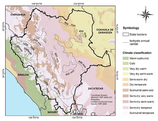
On the side of the Pacific, region running from the Northwest to the Southwest, is the region with the highest precipitation (mean annual precipitation 1,200 mm), coinciding with the forest and rainforest areas of Durango. In this part of the state is the Sierra Madre Occidental, where humidity from the Pacific Ocean condenses as it ascends creating the most important rain events.
Just a small part of the humidity from the Pacific passes over the orographic barrier onto the inland slope of Durango to the grassland, shrub, and agriculture area. Here, the mean annual precipitation is 600 mm, becoming lower as it moves eastward to a mean annual precipitation of 200 mm, presenting semi-dry, dry, and very dry climates (SEMARNAT, 2009).
Meteorological information
The meteorological information of the maximum and minimum temperatures and precipitation at a daily scale from the meteorological stations located in the study area was collected from the databases of the National Meteorological Service (SMN). The monthly information per station was downloaded from smn.cna.gob.mx/es/climatologia/informacion-climatologica.
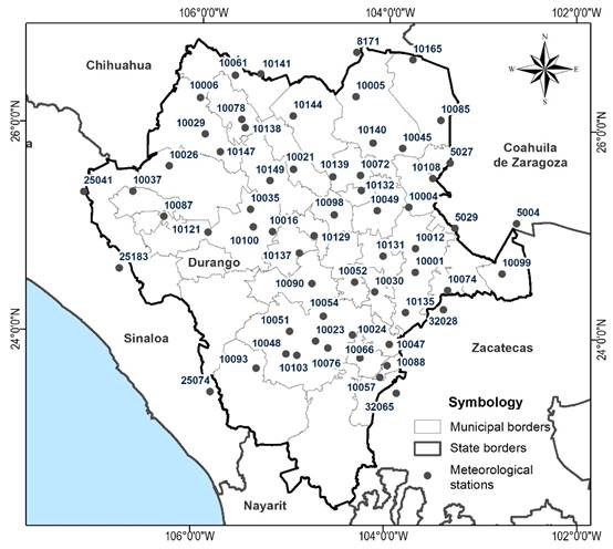
The study period chosen is from 1979 to 2008, as it includes the highest number of stations with registries (with at least 90%, some with 75% registries in areas with little information) during the study period. A total of 61 meteorological stations of the SMN were used, 52 of which belong to the state of Durango, three to Coahuila, three to Sinaloa, two to Zacatecas, and one to Chihuahua (Figure 3).
The meteorological information was subjected to a data quality control consisting of identifying unreasonable values according to the criteria: (1) precipitation values under zero and (2) Maximum daily temperature below the minimum daily temperature. The unreasonable values were eliminated and treated as missing data.
The missing data were completed in two ways: (1) the U.S. National Weather Service (NWS) method, also known as the inverse distance squared. This is an easy-to-use method, but one must have the information from nearby stations (Campos, 1998). It can be applied to daily, monthly, or annual data. Recent works indicate that it is one of the best methods to estimate missing data in Mexico ((Gallegos, Arteaga, Vázquez, & Juárez, 2016; Gamboa, 2015). (2) The Climate Forecast System Reanalysis (CFSR) developed by the National Center for Environmental Prediction (NCEP) and the National Center for Atmospheric Research (NCAR) of the United States of America. It is a model that represents the global interaction between the oceans, the ground, and the atmosphere (Saha et al., 2010). It encompasses 35 years (1979-2014) of daily data for temperature, precipitation, wind, relative humidity, and solar energy variables. The resolution of the CFSR is approximately 38 km (Saha et al., 2014).
The NWS method estimates the missing value of a station according to the following equation:
Where Pi is the observed precipitation in the auxiliary station i; I = 1, 2, 3…n, for the missing date; n is the number of auxiliary stations (minimum n = 2).
Di is the distance between each auxiliary station and the incomplete station, in km.
For each station, the closest stations were located as auxiliaries and their distances were calculated. When possible, the four nearest stations were located; one to each quadrant of the North-South and East-West axes (Campos, 1998).
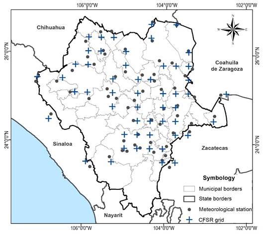
The data of the CFSR model were obtained from the website: globalweather.tamu.edu. The point grid data for the state of Durango were downloaded. To complete the missing data, the nearest grid point to each meteorological station was chosen (Figure 4).
The missing data for 59 stations were completed with the procedure more adequate method for each variable. To do this, the explicative capacity of the models was evaluated for the data measured in the meteorological stations through five statistical indices: mean square error (MSE) (Sánchez-Algarra, Barraza-Sánchez, Reverter-Comas, & Vegas-Lozano, 2006) root-mean-square error (RMSE) (Lehmann & Casella, 1998), mean absolute error (MAE) (Fuertes & Javier, 1998), Willmott index (d) (Willmott, 1982), and the determination coefficient (R 2) (Infante & Zarate, 2012).
Each index has a criterion to determine if the model is a good estimator; this way the better method was chosen to estimate the missing data: that in which at least three statistical indices highlighted it as the better estimator.
The CFSR model was the better estimator of lost data regarding maximum temperature in 34 stations, compared with the 25 stations completed with the NWS method. The NWS method is the better estimator for precipitation as it was evaluated as better in 57 stations, while the CFSR model was better in only two of them. For minimum temperature, the NWS method was better in 41 stations. Accordingly, 61 complete monthly climatic series were obtained for the maximum and minimum temperatures, and precipitation variables.
Methodology
Drought index
The Standardized Precipitation Index (SPI) and Standardized Precipitation Evapotranspiration Index (SPEI) indices were used for the drought analysis. According to the recommendations by the World Meteorological Organization (OMM, 2016), these have been previously tested in this area of study (Rivera, Crespo, Arteaga, & Quevedo, 2007; Llanes et al., 2018), and they can be used according to the available data.
The SPI was developed by McKee, Doesken, and Kleist (1993) with the objective of quantifying the impacts of precipitation deficit on the different hydrological resources: underground water, stored water, waterways, and soil humidity. The index is defined based on standardized precipitation, which is the difference of the mean precipitation for a specific timeframe divided by the standard deviation where the mean and the deviation are determined from past registries.
It is calculated based on a set of monthly precipitation data, which is always moving as in each month a new value is determined from the prior months. Each of the datasets is adjusted to the Gamma function to define the relationship between the probability and the precipitation. Given that the Gamma function in climatic analyses is the integral, obtained from the probabilities of a precipitation happening that is lower than or equal to a determined precipitation volume. In order to facilitate the obtention of the SPI index, the accumulated probability is transformed into a normalized Z variable (with mean = 0, and variance = 1), that represents the SPI value.
The SPEI was developed by Vicente, Beguería, and López (2010). It is a multi-scale drought index that combines precipitation and temperature data, and works based on the original SPI calculation procedure. The SPEI uses the monthly (or weekly) difference between precipitation and evapotranspiration (PET). This represents a simple climatic water balance fixed at different time scales to obtain the SPEI.
Calculating the PET is difficult due to the number of parameters intervening in the process. The goal of including the PET in the calculation of the drought index is to obtain a relative temporal estimation and therefore, the method used to calculate the PET is not critical. This is to say, the SPEI is not linked to any particular method.
To calculate the SPEI, a three-parameter distribution is needed since it can have negative values, common in the balance series between precipitation and evapotranspiration. Vicente et al. (2010) selected the Log-logistic probability density function based on the behavior of of the most extreme values. Subsequently, it is transformed to a standard normal distribution with mean = 0 and variance = 1. Given that the SPEI is a standardized variable, it can be compared against other SPEI values throughout time and space.
Mckee et al. (1993) used a classification system to define drought intensities (Table 1), and defined criteria for when a drought even happens in any time scale. Since the SPEI is a standardized variable, as is the SPI, the same drought classification system is used for both indices.
Table 1 SPI and SPEI classification.
| Index value | Index category |
|---|---|
| 2 or higher | Extremely humid |
| 1.5 to 1.99 | Very humid |
| 1.0 to 1.49 | Moderately humid |
| -0.99 to 0.99 | Near Normal |
| -1.0 to -1.49 | Moderately dry |
| -1.5 to -1.99 | Very dry |
| -2 or lower | Extremely dry |
The SPEI and SPI indices were calculated for the climatic series using the RStudio® program (RStudio Inc., 2018) with the SPEI software (Beguería, Serrano, & Sawasawa, 2013). The SPEI and SPI indices were obtained at 6- and 12-month scales. Besides maximum and minimum temperature and precipitation climatic information, the latitude of each station was also used. The Hargreaves method was selected to estimate evapotranspiration.
Normality test
The Rodionov method uses the t-student test as part of the procedure to detect changes.
To use the t test procedure, the assumption must be met that the data come from a normal distribution (Montgomery, 2010).
To test the normality of the data, the Kolmogorov-Smirnov goodness of fit test was chosen, as modified by Lilliefors (1967). The test was applied to each drought index series using the nortest software in RStudio®, with a significance level (alpha, α) of 0.01.
Rodionov method to detect regime shifts
Rodionov (2004) proposed a sequential method to detect regime shifts (in the mean and standard deviation) as a solution to the problem of temporal series that do not take into account the final data from existing methods for the detection of a regime shift, and which consequently are detected much after their real appearance.
The method consists of doing a test to determine the validity of the null hypothesis H 0 (in this case, the existence of a regime shift). There are three possible results of the test: accepting H 0 , rejecting H 0 , or continue doing the test.
In a time series, when a new observation arrives, which happens regularly, a test is done to determine if it represents a statistically significant deviation of the mean value of the current regime. If it does, that year is marked as a possible point of change c, and the subsequent observations are used to confirm or reject this hypothesis (Rodionov & Overland 2005).
The hypothesis is proven when using the regime shift index (RSI) which is calculated for each c:
Where m = 0, …, l - 1 is the number of years since the beginning of a new regime, l is the cut length of the regimes to be tested, and σ
l
is the mean standard deviation for all the intervals of a year in the time series. RSI represents a cumulative sum of normalized deviations x
i
* of the hypothetic mean level for the new regime (
Where t is the value of the t-student distribution with 2l - 2 degrees of freedom at a given level of probability p. If, at any moment from the beginning of the new regime, the RSI becomes negative the test fails and a value of zero is assigned. If the RSI remains positive during l - 1, then c is explained as the time of a regime shift at level ≤ p. The search for the next regime shift begins with c + 1 to guarantee that its synchronization is correctly detected, even if the real duration of the new regime is < 1 year.
The mean value of the current regime
The changes in variance of any meteorological variable can have a similar or even greater impact on the ecosystems than changes in the mean. Like climatic changes due to natural or human causes, they can be changes in the frequency of extreme events that represent the danger of favoring an increase of global warming (Rodionov, 2005b).
Rodionov developed an extension for Excel (Rodionov, 2005b) that detects changes in variance. This procedure is similar to that of the mean, except that it is based on the F test instead of the t test.
The entry data for the program are the values of the drought indices and the parameters of the test: cut length, level of significance, and the Huber weight function.
The cut length and level of significance parameters control he magnitude and the scale of the detected regimes. Different combinations in these parameters have a direct effect on the RSI value; this is to say, there will be different interpretations of the results (Rodionov, 2006a). Thusly, we analyzed the case of a cut length of 5 for a significance level of 0.05. The Huber weight parameter controls the participation of atypical values. Because of these values, the mean is not representative of the mean value of the regimes. The weight for the value of the data must be chosen so that it is small if this value is considered an atypical value (Rodionov, 2006a). In function of the standard deviation, we used a Huber weight of 2.
Analysis of change trends in the mean and variance of the drought indices
For each station, we calculated the frequencies of occurrence of changes in the mean (RSI) and variance (RSSI) of the drought indices. For the RSI values, we calculated only the frequency of the negative RSI values, which represent drought regimes.
A spatial analysis of the frequencies obtained from the RSI and RSSI values was done through interpolation based on the principle of autocorrelation to determine if there is a spatial pattern (Childs, 2004). The interpolation was done with the Spatial Analyst extension of ArcGIS® (ESRI, 2016) with the kriging method (Villatoro, Henríquez, & Sancho 2008).
For the trend analysis, the frequencies of the occurrence of changes in the mean and variance were grouped into five- and ten-year periods. We identified whether during these periods there was a trend to decrease or increase the number of changes.
Results
The SPEI and SPI drought indices were calculated for 6 months in the period from June 1979 to December 2008. For the SPEI and SPI indices for 6 months the values obtained go from December 1979 to December 2008. Table 2 shows the statistics of the drought indices.
Table 2 General statistics of the drought statistics for the state of Durango, Mexico.
| Drought index | Mean | Standard deviation | Minimum | Maximum | Range |
|---|---|---|---|---|---|
| 6 month SPI | 0.009 | 0.984 | -3.025 | 2.46 | 5.485 |
| 12 month SPI | 0.003 | 0.986 | -2.752 | 2.376 | 5.128 |
| 6 month SPEI | 0.008 | 0.979 | -2.308 | 2.268 | 4.576 |
| 12 month SPEI | 0.006 | 0.978 | -2.157 | 2.161 | 4.318 |
The mean of the indices (SPI and SPEI) is very near zero, which indicates that the extreme values (periods of drought and humidity) occur with the same frequency. This means that the presence of droughts during the study period is a normal characteristic of the climate in the region this result is similar to that reported by Contreras (2005).
In terms of the magnitude of the means of extreme values, it is greater for the minimum values in three of the analyzed indices (6 and 12 month SPI and 6 month SPEI). This indicates that the magnitude of the drought is greater than the magnitude of the humid periods. This translates as droughts representing a higher risk for the area when they do happen.
Regarding the normality tests, they were met in: 46 stations for the 6 month SPI, 45 for the 6 month SPEI, 32 for the 12 month SPI, and 31 for the 12 month SPEI. The Rodionov test to detect regime shifts was done for the 6 month SPI and SPEI indices, as they are the ones that have a greater number of stations that met the normality test. This was done in order to include a larger surface area in the analysis.
Analysis of regime shift in the mean (RSI) and variance (RSSI)
For the mean of the 6 month SPI and SPEI indices, we obtained the RSI, the mean of the regimes with equal weights, the mean value of the regimes calculated with the Huber weight function, the length of the regimes, the final confidence level of the changes and the weight (in function of the standard deviation) of the atypical values.
For the variance, we obtained the regime shift index of the mean variance (RSSI), and like for the mean, we obtained the length of the regime and the confidence level for the changes.
With the RSI and RSSI values, the frequencies of occurrence for the change values per station were calculated for the 1979-2008 period.
For the RSI, we obtained the frequencies of the negative values, which indicate a shift towards a drought regime. The minimum and maximum RSI and RSSI values were obtained, respectively, for each station, as well as the date when they happened.
The minimum mean RSI values are -3.23 for the 6 month SPEI index, and -2.96 for the 6 month SPI. The mean maximum RSSI values are 1.30 for the 6 month SPEI, and 2.00 for the 6 month SPI.
With regard to the changes in the mean, there is a higher frequency of occurrence of maximum values on a specific date while in the case of changes in variance the frequency is more constant.
Through the spatial analysis, areas of the state were identified showing a higher frequency of regime shifts in the mean and variance. For RSI, in both indices the values of lowest occurrence are in the South of the State, which encompasses a larger area in the SPI index. One station, located in the Northwest, showed the highest frequency for the SPEI index, while for the SPI index, the RSI change frequency was the lowest (Figure 5).

Figure 5 Spatial distribution of the frequency of RSI values during the 1979-2008 period in the state of Durango, Mexico.
Figure 6 shows that the frequency of change values in the RSSI variance ranges from 5 to 13 during the 1979-2008 period. For the 6 month SPEI, the lowest frequency is to the West of the State, in the shape of a strip running from North to South, excluding a small portion on the borders with Chihuahua and Sinaloa, which shows a frequency of 7 to 9 occurrences. The same is true for most of the state since the higher frequencies only represent a small area to the East, corresponding to the values of only two climatological stations.
The RSSI frequency for the 6 month SPI index showed two categories of occurrence: from 7 to 9 covering most of the State, and from 9 to 11 distributed to the West (resulting from two stations) and a small portion to the East (from one station).
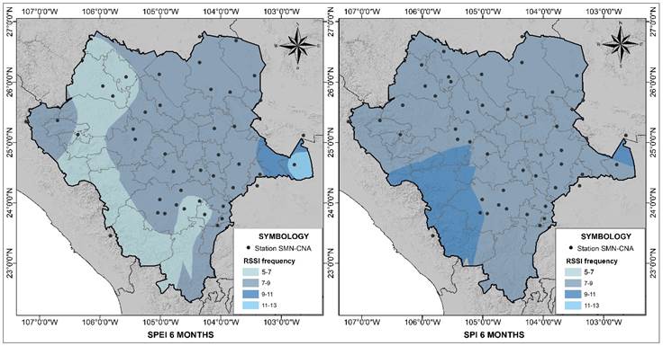
Figure 6 Spatial distribution of the frequency of RSSI values during the 1979-2008 period in the state of Durango, Mexico.
The detection of changes in the mean and variance depends on the drought index used. When using the SPEI index, the frequencies show greater variability by grouping in a higher number of categories than the frequencies obtained for the SPI index.
According to the spatial analysis, the North region of the State shows a higher frequency of changes, being 10078 Sardinas the station that shows the highest number of changes.
Due to the aforementioned, below is presented an individual analysis of the results obtained from this station for the RSI and RSSI values (changes in the mean and variance of the drought indices respectively).
The graphs (Figure 7) show the values of the drought indices, as well as the RSI and RSSI values. The negative RSI values were placed at the beginning of the drought periods for the 6 month SPEI and SPI indices. This means that the method detected all the shifts towards a drought regime.
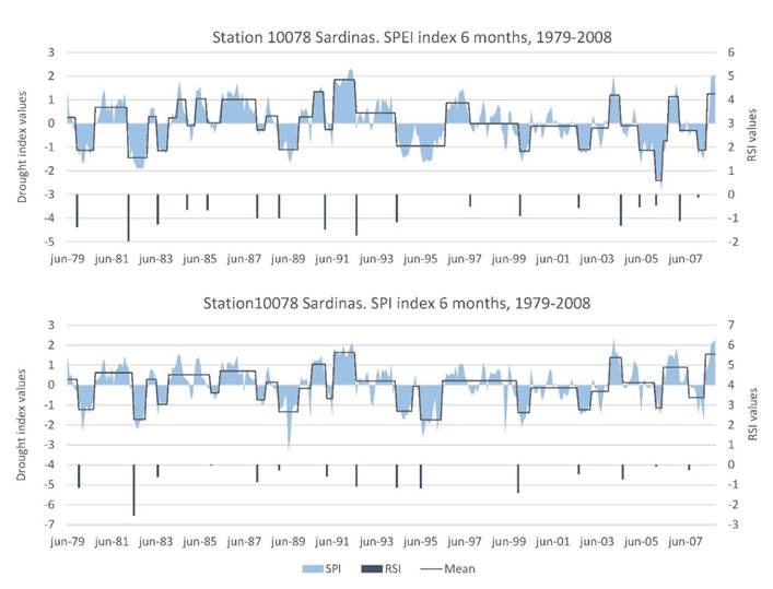
There were 18 changes in the mean for the 6 month SPEI index and 16 changes for the 6 month SPI index. Most of the RSI values were calculated on the same dates for both indices. The detection of changes in the mean thus depends on the drought index that is used (SPEI or SPI), it being more sensitive with the SPEI index.
Between 1994 and 1996 was the greatest drought period in the 10078 Sardinas station. Two negative changes in the mean are seen during this period. Thusly, the RSI value is useful to detect if a drought will continue, as the negative RSI value indicates that the drought classification values of the indices will continue in the same trend.
Higher RSI values are obtained when the regime shift is more abrupt while when the mean is more constant, the shift happens more gradually and the RSI values are lower. If the drought indices are in the higher values for humidity (positive) or drought (negative) the change to a high value in the opposing condition results in higher RSI values.
The maximum RSI values occurred on diverse dates in the analyzed stations however, we detected that a large part of them happened from June to July 1992.
The changes in variance do not indicate a general behavior of drought, but rather it is specific to the index used. Moreover, variance is sensitive to extreme values making the interpretation of the results skew to a rapid change in the values of the drought indices.
The detected changes in variance for station 10078 Sardinas (Figure 8) show a constant mean variance in practically the whole period. For the 6 month SPEI, the changes in variance are from 1985 to 1987, while for SPI, most of the changes were detected at the end of the series, from 2005 to 2007.
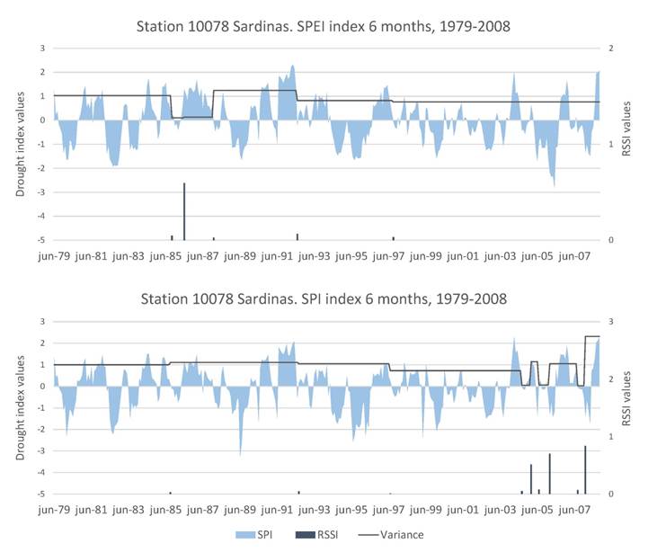
In station 10078 Sardinas, the maximum RSSI values do not coincide with the maximum RSI values, rather the maximum RSSI are observed in a variation of the mean of the drought indices. This is to be expected, as the variance index indicates the dispersion of the values with respect to the mean.
Given the aforementioned, we can infer that the RSSI values will be useful to detect shifts towards a prolonged drought period. Nevertheless, when the humid periods alternate with the drought periods with the same magnitude and duration, no changes in variance will be detected. Therefore, the RSSI values must be used as a complement of the RSI values. With both tests, it is possible to more accurately detect prolonged and more severe drought periods.
The frequency of the RSI and RSSI change values of the mean and variance in the drought indices were analyzed through the sum of values every five and ten years. In this way, we identified the trend of the shift frequency; this is, if the occurrence of changes in the mean and variance of the drought indices has increased or decreased through time.
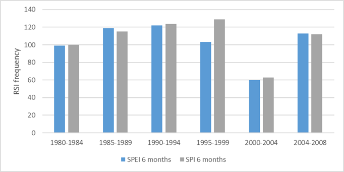
The trend of the frequency of changes in the mean every five years (quinquennial) for the six month SPEI and SPI drought indices is shown in Figure 9. The frequency of both indices is similar, only in the 1995-1999 period is the frequency of changes for the six month SPEI index lower than for the 6 month SPI index. During the first four quinquenniums, there is an increasing trend in the changes in the mean, which then decreases radically in the 2000-2004 period. In the last period, 2004-2008, the changes increase again up to values similar to those in the first quinquenniums.
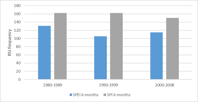
The frequencies of changes in the mean every ten years (decennial) in the graph (Figure 10) shows that in the last decade (2000-2008) had the lowest number of changes, while the 1990-1999 period showed the highest frequency of RSI values.

The obtained results coincide with those found buy Llanes et al. (2018), where they conclude that extreme drought events happened during 1990 and 1997, with the intervening years being a period of recurring droughts.
Figure 11 shows the frequency of changes in variance for the 6 month SPI and SPEI drought indices. There we can see a higher frequency (>40) of changes for the 6 month SPI index in all the periods, where the RSSI frequency is higher for SPI than for SPEI.

The frequency of changes in variance for ten year periods is shown in Figure 12. We can see that the first decade of the analysis (1980-1989) showed the highest frequency of changes; however, the SPI value is repeated in the following decade so the mean of changes during those 20 years was relatively constant.
The results obtained indicate that the changes in the mean and variance have not been greater in the last years of the analyzed period.
Conclusions
Drought was analyzed through the SPI and SPEI drought indices at 6 and 12 month timescales in the State of Durango. The drought periods were identified with the negative change values of the mean (RSI). We detected 14 mean changes for the 6 month SPEI index and 13 changes for the 6 month SPI index. The values of change in variance (RSSI) numbered 8 for the 6 month SPEI index, and 10 for the 6 month SPI index.
The trends of the changes in the mean and variance of the drought indices based on the frequency of changes in the mean decreased during the 2000-2004 period and increased during 2005-2008. The decade with the greatest changes in the mean was 1990-1999. In the case of variance, the maximum frequency of changes was during the 1985-1989 period, and the changes remained constant for the last 20 years. The decade with the greatest changes in variance was 1980-1989.
Referencias
Bates, B. C., Kundzewicz, Z. W., Wu, S., & Palutikof, J. P. (2008). Climate change and water. Climate Change and Water. DOI:10.1016/j.jmb.2010.08.039 [ Links ]
Begueria, S., Serrano, V., & Sawasawa, H. (2013). SPEI: Calculation of Standardised Precipitation-Evapotranspiration Index. R package version 1.6. DOI:10.1175/2009JCLI2909.1.http [ Links ]
Campos, D. F. (1998). Procesos del ciclo hidrológico. San Luis Potosí, México: Universidad Autónoma de San Luis Potosí. [ Links ]
Cancelliere, A., & Salas, J. D. (2010). Drought probabilities and return period for annual streamflows series. Journal of Hydrology, 391(1-2), 77-89. DOI:10.1016/j.jhydrol.2010.07.008 [ Links ]
Cenapred, Centro Nacional de Prevención de Desastres. (2002). Fascículo sequías. México, DF, México: Secretaría de Gobernación. Recuperado de http://www.cenapred.gob.mx/es/Publicaciones/archivos/8-FASCCULOSEQUAS.PDF [ Links ]
Childs, C. (2004). Interpolating surfaces in ArcGIS spatial analyst. Education Service. ArcUser July-September. 32-34 p. Recuperado de http://www.esri.com [ Links ]
Contreras, C. S. (2005). Las sequías en México durante el siglo XIX. Investigaciones Geográficas, (56), 118-133. Recuperado de http://www.scielo.org.mx/pdf/igeo/n56/n56a8.pdf [ Links ]
Domínguez, J. (2016). Revisión histórica de las sequías en México: de la explicación divina a la incorporación de la ciencia. Tecnología y ciencias del agua, 7(5), 77-93. [ Links ]
ESRI, Environmental Systems Research Institute. (2016). ArcMap | ArcGIS Desktop 10.5. Versión 10.5.0.6491. USA: Environmental Systems Research Institute, Inc. [ Links ]
Fuertes, S. J., & Javier, S. (1998). Evaluación de dos métodos de determinación de la evapotranspiración de referencia en condiciones semiáridas. Recuperado de http://hdl.handle.net/10261/16644 [ Links ]
Gallegos, J., Arteaga, R., Vázquez, M. A., & Juárez, J. (2016). Estimation of missing daily precipitation and maximum and minimum temperature records in San Luis Potosí. Ingeniería Agrícola y Biosistemas, 8(1), 3-16. DOI: 10.5154/r.inagbi.2015.11.008 [ Links ]
Gamboa, R. O. (2015). Evaluación de modelos empíricos, matemáticos y redes neuronales para estimar datos faltantes en estaciones meteorológicas en México (tesis de maestría en ciencias), Postgrado de Hidrociencia, Colegio de Postgraduados. [ Links ]
Heim, R. R. (2002). A review of twentieth-century drought indices used in the United States. Bulletin of the American Meteorological Society, 83(8), 1149-1165. DOI: 10.1175/1520-0477(2002)083<1149:AROTDI>2.3.CO;2 [ Links ]
Hounam, C. E., Burgos, J. J., Kalik, M. S., Palmer, W. C., & Rodda, J. (1975). Drought and agriculture (Technical Note No. 138). World Meteorological Organization, (392), 129. [ Links ]
Ibarrarán, M. E., & Rodríguez, M. (2007). Estudio sobre economía del cambio climático en México. Recuperado de http://inecc.gob.mx/descargas/cclimatico/e2007h.pdf [ Links ]
INEGI, Instituto Nacional de Estadística y Geografía. (2017). Anuario estadístico y geográfico de Durango 2017. Recuperado de http://internet.contenidos.inegi.org.mx/contenidos/Productos/prod_serv/contenidos/espanol/bvinegi/productos/nueva_estruc/anuarios_2015/702825077174.pdf [ Links ]
Infante, S., & Zarate, G. P. (2012). Métodos estadísticos. Un enfoque interdisciplinario (3a ed.). Colegio de Postgraduados. España: Mundi-Prensa. [ Links ]
Lehmann, E. L. & Casella, G. (1998). Theory of point estimation. Springer Texts in Statistics (2nd ed.) New York, USA: Springer-Verlag Inc. [ Links ]
Lilliefors, H. W. (1967). On the Kolmogorov-Smirnov Test for Normality with Mean and Variance Unknown. Journal of Statistical Association, 62(318), 399-402. DOI: 200.130.19.152 [ Links ]
Llanes, O., Gaxiola, A., Estrella, R. D., Norzagaray, M., Troyo, E., Pérez, E., Ruíz, R., & Pellegrini, M. de J. (2018). Variability and factors of influence of extreme wet and dry events in Northern Mexico. Atmosphere, 9(4), 1-16. DOI: 10.3390/atmos9040122 [ Links ]
Mckee, T. B., Doesken, N. J., & Kleist, J. (1993). The relationship of drought frequency and duration to time scales. AMS 8th Conference on Applied Climatology, (January), 179-184. Recuperado de https://doi.org/citeulike-article-id:10490403 [ Links ]
Miller, A. J., Cayan, D. R., & Barnett, T. P. (1994). The 1976-77 climate shift of the Pacific Ocean. Oceanography, 7(1), 21-26. [ Links ]
Montgomery, D. C. (2010). Diseño y análisis de experimentos (2ª ed.). México, DF, México: Limusa Wiley. [ Links ]
OMM, Organización Meteorológica Mundial. (2016). Manual de indicadores e índices de sequía. Programa de gestión integrada de sequías. Recuperado de http://www.droughtmanagement.info/literature/WMO-GWP_Manual-de-indicadores_2016 [ Links ]
Ortega, D. (2013). Sequía : causas y efectos de un fenómeno global. Ciencia y Sociedad, 16(61), 8-15. Recuperado de https://www.researchgate.net/publication/260163188 [ Links ]
Rivera, R., Crespo, G., Arteaga, R., & Quevedo, A. (2007). Temporal and spatial behavior of drought in the state of Durango, Mexico. Terra Latinoamericana, 25(1), 383-392. [ Links ]
Rodionov, S. (2004). A sequential algorithm for testing climate regime shifts. Geophysical Research Letters, 31(9), 2-5. DOI: 10.1029/2004GL019448 [ Links ]
Rodionov, S. (2005a). A brief overview of the regime shift detection methods. In: Velikova, V., & Chipev, N. (eds.). Large-scale disturbances (regime shifts) and recovery in aquatic ecosystems: Challenges for management toward sustainability. UNESCO-ROSTE/BAS Workshop on Regime Shifts (pp. 17-24), 14-16 June 2005, Varna, Bulgaria. [ Links ]
Rodionov, S. (2005b). A sequential method for detecting regime shifts in the mean and variance. Joint Institute for the Study of the Atmosphere and Ocean. Seattle, USA: University of Washington. Recuperado de https://www.beringclimate.noaa.gov/regimes/rodionov_var.pdf [ Links ]
Rodionov, S. (2006a). Help with regime shift detection software. Recuperado de https://www.beringclimate.noaa.gov/regimes/help3.html [ Links ]
Rodionov, S. (2006b). Sequential regime shift detection. Recuperado de https://www.beringclimate.noaa.gov/regimes/ [ Links ]
Rodionov, S., & Overland, J. (2005). Application of a sequential regime shift detection method to the Bering Sea ecosystem. Journal of Marine Science, 62(May), 328-332. DOI: 10.1016/j.icesjms.2005.01.013 [ Links ]
RStudio Inc. (2018). RStudio. Recuperado de https://www.rstudio.com/products/rstudio/download/ [ Links ]
Saha, S., Moorthi, S., Pan, H.-L., Wu, X., Wang, J., Nadiga, S., Tripp, P., Kistler, R., Woollen, J., Behringer, D., Liu, H., Stokes, D., Grumbine, R., Gayno, G., Wang, J., Hou, Y. T., Chuang, H. Y., Juang, H. M. H., Sela, J., Iredell, M., Treadon, R., Kleist, D., Van Delst, P., Keyser, D., Derber, J., Ek, M., Meng, J., Wei, H., Yang, R., Lord, S., van den Dool, H., Kumar, A., Wang, W., Long, C., Chelliah, M., Xue, Y., Huang, B., Schemm, J. K., Ebisuzaki, W., Lin, R., Xie, P., Chen, M., Zhou, S., Higgins, W., Zou, C. Z., Liu, Q., Chen, Y., Han, Y., Cucurull, L., Reynolds, R. W., Rutledge, G., & Goldberg, M. (2010). The NCEP Climate Forecast System Reanalysis. Bulletin of the American Meteorological Society, 91(8), 1015-1058. DOI:10.1175/2010BAMS3001.1 [ Links ]
Saha, S., Moorthi, S., Wu, X., Wang, J., Nadiga, S., Tripp, P., Behringer, D., Hou, Y. T., Chuang, H. Y., Iredell, M., Ek, M., Meng, J., Yang, R., Peña-Mendez, M., van den Dool, H., Zhang, q., Wang, W., Chen, M., & Becker, E. (2014). The NCEP Climate Forecast System Version 2. Journal of Climate, 27(6), 2185-2208. DOI: 10.1175/JCLI-D-12-00823.1 [ Links ]
Sánchez-Algarra, P., Barraza-Sánchez, X., Reverter-Comas, F., & Vegas-Lozano, E. (2006). Métodos estadísticos aplicados. Barcelona, España: Universitat de Barcelona. [ Links ]
Semarnat, Secretaría de Medio Ambiente y Recursos Naturales. (2009). Programa Hídrico Visión 2030 del Estado de Durango. México, DF, México: Secretaría de Medio Ambiente y Recursos Naturales. [ Links ]
Vicente, S. M., Beguería, S., & López, J. I. (2010). A multiscalar drought index sensitive to global warming: The standardized precipitation evapotranspiration index. Journal of Climate, 23(7), 1696-1718. DOI:10.1175/2009JCLI2909.1 [ Links ]
Villatoro, M., Henríquez, C., & Sancho, F. (2008). Comparación de los interpoladores idw y kriging en la variación espacial de ph, ca, cice y p del suelo. Agronomia Costarricence, 32(1), 95-105. [ Links ]
Willmott, C. J. (1982). Some comments on the evaluation of model performance. American Meteorological Society, 63(11), 1309-1313. DOI: 10.1175/1520-0477(1982)063<1309:SCOTEO>2.0.CO;2 [ Links ]
Received: November 24, 2018; Accepted: March 27, 2019
 Este es un artículo publicado en acceso abierto bajo una licencia Creative Commons
