


Serviços Personalizados
Journal
Artigo
 texto em
  Inglês (pdf)
 Artigo em XML
 Referências do artigo
 Enviar este artigo por email
Indicadores
-
 Citado por SciELO
 -
 Acessos
Links relacionados
-
 Similares em
SciELO
Similares em
SciELO
Compartilhar

 Permalink
Tecnología y ciencias del agua
versão On-line ISSN 2007-2422
Tecnol. cienc. agua vol.10 no.6 Jiutepec Nov./Dez. 2019 Epub 15-Maio-2020
https://doi.org/10.24850/j-tyca-2019-06-05
Articles
Geometric optimization of a submerged lens for wave energy focusing

1División Ambiental, AECOM México-DCS Américas, Ciudad de México, México, santiago.gaja@aecom.com
2Instituto de Ingeniería, Universidad Nacional Autónoma de México, Ciudad de México, México, emendozab@iingen.unam.mx.
3Instituto de Ingeniería, Universidad Nacional Autónoma de México, Ciudad de México, México, rsilvac@iingen.unam.mx.
Abstract In this paper, the use of submerged structures of elliptical form are proposed as a viable alternative to focusing of the swell and with it to have high energy sources for its use as a source of renewable energy. A numerical model, validated with experimental data, was used to determine the optimal geometry of the submerged elliptical structure in terms of the length and direction of the incident wave. The results allow the design of the submerged elliptical lenses to function in local hydrodynamic conditions to obtain maximum performance and offer metrics of their efficiency for different geometries in terms of their eccentricity, height, and depth of installation.
Keywords CELERIS; energy focalization; submerged lenses; wave energy
En este trabajo se propone el uso de estructuras sumergidas de forma elíptica como una alternativa viable para la focalización del oleaje y con ello disponer de focos de alta energía para su aprovechamiento como fuente de energía renovable. Se empleó un modelo numérico, validado con datos experimentales, para determinar la geometría óptima de la estructura elíptica sumergida en términos de la longitud y dirección del oleaje incidente. Los resultados permiten diseñar lentes elípticos sumergidos como función de las condiciones hidrodinámicas locales para obtener su máximo desempeño, y ofrece métricas de su eficiencia para distintas geometrías en términos de su excentricidad, altura, y profundidad de instalación.
Palabras clave CELERIS; focalización de energía; lentes sumergidos; energía del oleaje
Introduction
The efficiency of submerged lenses to focus wave energy has been studied by mathematicians and engineers for more than 30 years. Various geometric shapes have been analyzed to evaluate their ability to amplify the waves in a determined, or focal, point and thus provide a useful tool in terms of energy capture and coastal protection.
The first theoretical and experimental studies involved a Fresnel-type lens to produce a non-uniform phase change in a diverging wave to transform it into a converging wave (Mehlum & Stamnes, 1987; Stamnes, Lovhaugen, Spjelkavik, Chiang, & Yue, 1983). Murashige and Kinoshita (1992), made a comparative study between a Fresnel lens and a biconvex lens, both using a profile constructed of small cylinders to reduce the effects of wave reflection. The results showed that biconvex lenses have a better performance than Fresnel lenses, and that using an arrangement of small cylinders as a profile improves efficiency.
A more recent investigation, with more significance to the present project, was the comparative numerical study on the efficiency of a biconvex lens and an elliptical lens, by Griffiths and Porter (2011). In this work, a region of shading around the lenses was included to reduce the effect of diffraction that contributes negatively in the focusing process. The refraction theory was used in conics, to obtain a controlled and predictive targeting process, as this theory establishes that any beam of light that falls parallel to the optical axis of an ellipsoid with a refractive index inverse to the eccentricity (
Therefore, for a given frequency and starting from a known depth
This paper is divided as follows, in section 2 the methodology used to carry out the numerical evaluation of the elliptical lens is described. This was carried out by means of a wave model of Boussinesq type, which was validated from laboratory tests in the wave basin of the Engineering Faculty of the UNAM (FI-UNAM). The results about the validation of the numerical model of Boussinesq as well as the numerical evaluation of the performance of the elliptical lens as a function of its geometrical parameters and the incident waves, are shown in section 3. Finally, in section 4 the most relevant conclusions of the present investigation.
Materials and methods
Numerical model
To carry out the numerical evaluation of the performance of the elliptical lenses, a wave model called CELERIS (Tavakkol & Lynett, 2017) was used, which solves the extended Boussinesq equations (Madsen & Sorensen, 1992). This type of equation solves the physical processes of refraction, diffraction, reflection, subjection and nonlinear interactions of waves in shallow water or in interaction with structures and is therefore suitable to solve coastal hydrodynamic processes (Nwogu, 1993; Kirby, 2003; Briganti, Musumeci, Bellotti, Brocchini& Foti, 2004), or interaction of waves with floating or submerged structures (Prinos, Avgeris, & Karambas, 2005; Fuhrman, 2005, Bingham, & Madsen, 2005; Soares & Mohapatra, 2015), and wave focusing processes (Tavakkol & Lynett, 2017). The numerical model was validated for different reference standard cases, such as wave run-up on slopes and conical islands, and wave focusing with circular geometries (Tavakkol & Lynett, 2017).
The equations involved are:
Where
In which
Experimental design to validate the CELERIS model
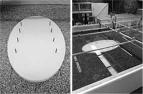
For the evaluation of the model in simulating the focusing process with elliptical lenses, experiments were conducted in the FI-UNAM, in a rectangular concrete structure with a maximum capacity of 37.72m3 of the following dimensions: 10.7 m long, 4.7 m wide and 0.75 m high (Figure 1). The swell was generated by a unidirectional, flap type paddle. A physical model of an elliptical lens with a semi-axis of less than 0.6 m, a half-axis greater than 1 m and a height of 0.122 m (Figure 2) was installed. A unidirectional monochromatic wave field was generated, with a frequency of 1.61 Hz and a height of 0.013 m. This was measured at the free surface, with resistive type level sensors. It should be noted that the dimensions of the elliptical lens were determined by numerical tests, where the semi-minor axis was fixed at the same value as the incident wavelength (
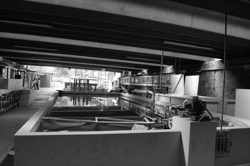
Figure 1 Rear view of the wave basin of the Hydraulics Laboratory of the Faculty of Engineering of the UNAM.
To simulate the transition from deep to shallow water, a horizontal platform was constructed with the same material as the dissipative beach, with a height of 0.13 m above the tank bottom. The water level in all the experiments was 0.35 m.
To record the focusing process, 2 transects were instrumented (Figure 3), one on the optical axis (transect AB) and another transverse to the optical axis on the focal point (transect CD).
To measure the perturbed waves on one side of the elliptical lens, three transects were instrumented parallel to the optical axis at the height of the ellipse (transects EF, GH and IJ).
In order to verify the operation of the model for oblique waves, and because the paddle only generates unidirectional waves, the lens was turned 20 ° on the optical axis to simulate oblique incidence. In the lower panel of Figure 3 a diagram of the position of the elliptical lens for oblique waves is shown, as well as the arrangement of the instruments which recorded changes in the focal area due to the change of the incident wave direction (KL and MN transects).
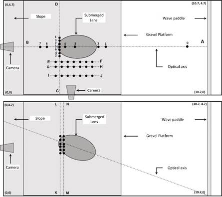
Figure 3 Diagram of the instrument arrangement for normal wave incidence (upper) and oblique (lower) incidence. The black dots represent the positions of the level sensors and the dotted lines represent the transects. The numbering in the upper panel indicates the comparison of the free surface and spectral time series.
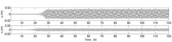
The free surface sampling frequency of the sensors was 100 Hz (0.01 s) and the time length of the record was 120 s for each test. Figure 4 shows an example of two series recorded during the measurement period. From the free surface time series, the temporal analysis was carried out by means of the zero down crossing method, in order to obtain the statistical wave parameters, such as the height H and the period T. Subsequently, the mean square height (
Where
In order to compare the amount of energy of the incident wave, the focused wave, and the wave at a control point (corresponding to the position of the wave at the focal point but without the lens), energy spectra were evaluated by means of the Fast Fourier Transform (FFT); which, from the record of the free surface in the time domain, gives the amount of energy as a function of the frequency.
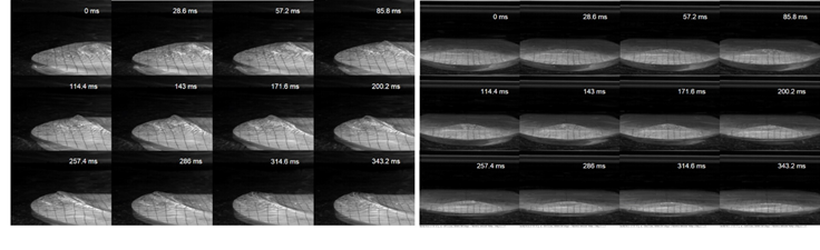
In addition to the surface level measurements recorded by the level sensors, the focusing process was recorded by means of a high-speed camera. The camera was installed in 2 positions, to record the side and front views of the focusing process (Figure 5). The video recording had a rate of 700 frames per second. Figure 5 shows a set of video frames for the case of normal incidence side view (upper panel) and front view (lower panel). For the case of side view, the waves travel from right to left, reaching a maximum in the focal area at 143 ms. In the front view, the transverse view of the lens is seen and the waves approach from back to front, reaching a maximum at 143 ms.
Numerical basin
To obtain the simulated free surface with the CELERIS model, a numerical replica of the FI-UNAM installation was used. The numerical domain was divided into cells, 536 by 236 for the length (10.7 m) and width (4.7 m) of the basin, respectively, giving a rectangular mesh with a spatial resolution of 0.02 m (Figure 6). Wave generation in the numerical basin was simulated by means of a periodic sine-type function with an amplitude of 0.0066 m, a period of 0.62 s and an 0° direction (perpendicular to the optical axis of the elliptical lens), on the eastern border. The variables
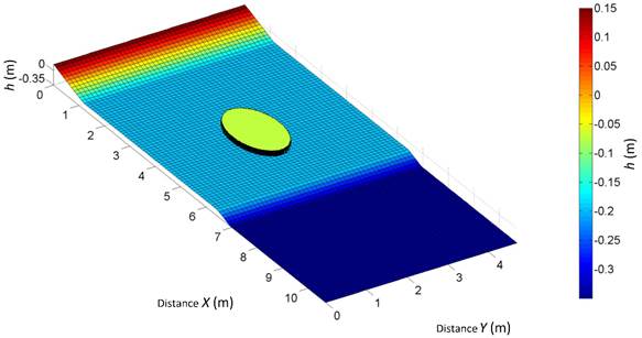
Figure 6 Schematic representation of the numerical basin used in the simulation of the focusing process with the CELERIS model. To visualize the discretization of the pond, each cell represents 5 cells of the numerical basin used.
To dissipate the wave energy and avoid reflection effects inside the numerical basin, the dissipative beach used in the physical modelling was replaced by a numerical sponge, which acts as a dissipation coefficient
Where Ls is the thickness of the sponge and D (x, y) is the normal distance to the absorbent boundary.
The side walls were considered totally reflective (as in the FI-UNAM), so that
For
The integration time step of the model's governing equations was 0.001 s, and the acquisition of results was 100 Hz to homogenize the recording frequency of the simulated free surface with that obtained in the FI-UNAM. The simulation time was 30 s for all the experiments. With respect to the processing of numerical results, the same methodology was followed as that for the physical modeling. First, time series of the free surface were obtained in the same position and sampling frequency as the level sensors used in the FI-UNAM (Figure 2) and then the
Results and discussion
The comparison of the free surface time series obtained with the CELERIS model and that of the experiments in the FI-UNAM, was made for a 10-second record, considering the 20 s as the beginning and 30 s as the end (Figure 7, left panel).
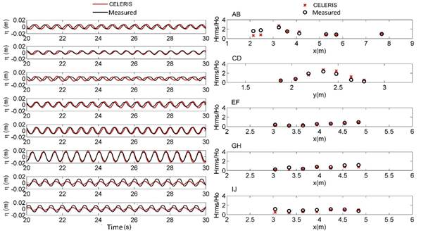
Figure 7 Left panel: Measured free surface data (black lines) and simulated, CELERIS model data (red lines). Right panel: Mean square heights: measured data (black circles) and CELERIS simulated data (red circles).
There was good agreement at the positions AB0, AB1, AB2, AB3, AB4 and AB5, but for the positions after the lens, AB6 and AB7, the model overestimated the measured data.
The positions that describe the focusing process on the lens are AB3, AB4 and AB5, where the latter has the greatest recorded amplitude. Positions AB2, AB1 and AB0, correspond to the positions before the lens.
For the evaluation of the elliptical lens performance, the most relevant information in the focalization process showed good agreement with the measured results (AB3, AB4 and AB5).
The standardized mean square height (
The transversal structure of the focal area (CD) was well represented by the model and the comparison of the waves in the lateral section to the lens (EF, GH and IJ) indicates that the model adequately represented the disturbed waves.
Figure 8 shows the comparison of
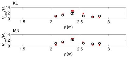
Figure 8 Comparison of the measured mean square height (black circles) and that simulated by the model (red crosses) on the KL and MN transects for the case of oblique incidence.
The comparison of
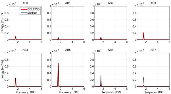
Figure 9 Comparison of the energy spectra obtained by means of simulations with the CELERIS model (red line) and from the recorded measurements (black line) on the AB transect.
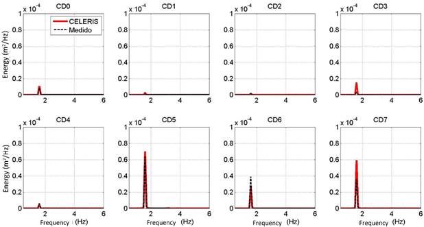
Figure 10 Comparison of the energy spectra obtained by means of CELERIS simulations (red line) and from that recorded in the FI-UNAM (black line) on the CD transect.
The comparison made by means of the free surface, the
Evaluation of the submerged lens performance
In order to standardize the performance tests in a reference parameter corresponding to the incident waves, the water depth, determined by the depth between the submerged lens and the water mirror
To obtain a comparison of the amplification of the energy, the spectrum was obtained for each test, at the focal point of the incident wave (at x = 8 m and y = 2.35 m) and at the control point. The focal point was defined as the location where the maximum
Because the waves in the basin can behave like a set of quasi-stationary waves (Dean & Darymple 1984), it is very important to know the influence of the reflected waves in the focusing process, especially if the experiments are prolonged (Cotter & Chakrabarti, 1994).
To know the influence of the energy reflected by the lateral walls of the numerical basin, two tests lasting 30 s were carried out in a basin with the lateral walls far away and in the basin validated for the same boundary conditions, to determine a window of time where the focus is not affected by reflection. Figure 11 shows the profile of
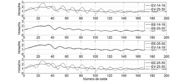
It can be seen that for the case of the validated basin (EV, first panel) there are significant differences in the profile of
Effects of the relative water depths of the submerged lens
The purpose of these tests was to evaluate the performance of the elliptical lens for different relations between
The platform on which the elliptical lens was mounted was fixed at a height of 0.15 m above the bottom of the numerical basin so that
Table 1 Position of the focus generated for different water strains. The obtained
| Test |
|
Pos. x (m) |
|
|
|
|
|---|---|---|---|---|---|---|
| WD1 | 1/3 | n/a | 0.0119 | 1.003 | n/a | |
| WD2 | ¼ | n/a | 0.0170 | 1.049 | n/a | |
| WD3 | 1/5 | 3.38 | 0.0231 | 1.104 | 0.02 | |
| WD4 | 1/6 | 3.38 | 0.0283 | 1.161 | 0.02 | |
| WD5 | 1/7 | 3.38 | 0.0317 | 1.219 | 0.02 | |
| WD6 | 1/8 | 3.38 | 0.0324 | 1.276 | 0.02 | |
| WD7 | 1/9 | 3.38 | 0.0306 | 1.332 | 0.02 | |
| WD8 | 1/10 | 3.62 | 0.0312 | 1.387 | 0.22 |
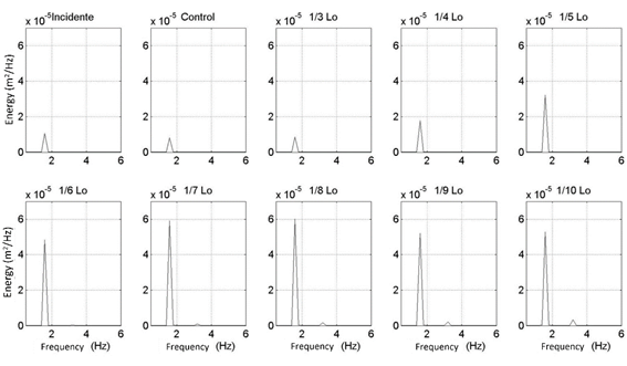
Figure 12 Energy spectra of the focalized wave for different water depths on the elliptical lens. The spectrum of the incident and control waves is shown.
As the water depth on the elliptical lens begins to decrease, the energy increases up to a maximum point in a depth of 1/8
For depths of 1/5
Eccentricity tests
Taking the numerical pre-tests, mentioned in the methodology, the semi major axis (a) remained fixed at a size of 1.7
Table 2 Position of the generated focus for different eccentricities. The obtained
| Test | Factor |
|
Pos. x (m) |
|
|
|---|---|---|---|---|---|
| LE1 | 1.500 | 0.484 | 3.140 | 0.0325 | 0.58 |
| LE2 | 1.064 | 0.784 | 3.380 | 0.0329 | 0.02 |
| LE3 | 1.000 | 0.811 | 3.380 | 0.0322 | 0.02 |
| LE4 | 0.875 | 0.859 | 3.380 | 0.0309 | 0.04 |
| LE5 | 0.750 | 0.899 | 3.380 | 0.0297 | 0.08 |
| LE6 | 0.500 | 0.956 | 3.440 | 0.0295 | 0.18 |
| LE7 | 0.375 | 0.975 | 3.440 | 0.0290 | 0.22 |
| LE8 | 0.250 | 0.989 | 3.700 | 0.0247 | 0.43 |
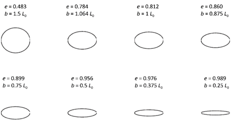
Figure 13 Different lens eccentricities for the numerical simulations. The eccentricity value (e) and the factor of 𝐿 0 by which the minor semi axis (b) was multiplied are shown.
In Figure 14, LE1, LE2 and LE3 are seen to have the highest amounts of concentrated energy, with values close to 6 times the incident energy and almost 8 times the energy observed at the control point. LE2 has the greatest increase. From LE4 the energy begins to decrease as the eccentricity increases until reaching the case of LE8.
It is important to note that in the tests of water depths and eccentricity, the cases determined by the law of conic refraction, are those that have most increased energy. For the case of water depth on the elliptical lens, the ratio of
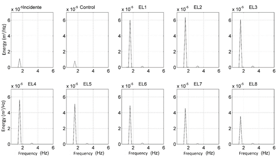
Figure 14 Energy spectra of the focalized wave for different eccentricities. The spectrum of the incident and control waves is shown.
For the case of the eccentricity tests, the eccentricity of the LE2 case was exactly the inverse of
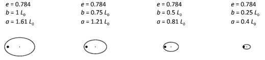
Figure 15 Schematization of the elliptical lenses used for the size optimization for a constant eccentricity of 0.784, obtained from the law of conic refraction.
Table 3 shows the position of each focus on the optical axis, the
Table 3 Position of the focus generated for the different sizes of the lens with constant eccentricity. The average quadratic height obtained in the focus is shown, as well as the size of the semi axes a and b, the area of the lens and the absolute distance between the numerical focus and the geometric focus
| Test |
|
|
|
Area (m2) |
|
|
|---|---|---|---|---|---|---|
| EC1 | 1.000 | 0.940 | 0.584 | 1.72 | 0.0330 | 0.02 |
| EC2 | 0.750 | 0.705 | 0.438 | 0.97 | 0.0329 | 0.02 |
| EC3 | 0.500 | 0.470 | 0.293 | 0.43 | 0.0276 | 0.08 |
| EC4 | 0.250 | 0.235 | 0.146 | 0.11 | 0.0181 | 0.14 |
Figure 16 shows the energy spectra obtained for each of the tests mentioned in Table 3, as well as for the incident wave and at the control point.
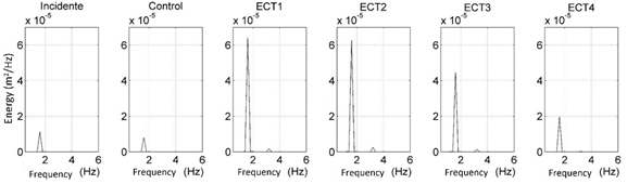
Figure 16 Energy spectra of the focalized wave for different sizes of elliptical lens for a constant eccentricity of 0.784. The spectrum of the incident and control waves is shown.
It can be observed in Figure 16 that despite the difference in size of the elliptical lenses corresponding to EC1 and EC2, both amplify approximately the same amount of energy, indicating that EC2 (with a semi axis of –
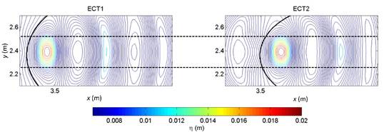
Tests of the total depth
In order to know how much the focusing process is affected by the elliptical lens with respect to the total depth in which it is submerged, several numerical simulations were performed for different depths. Table 4 shows the list of tests performed. Each test was given the acronym PP denoting Platform Depth. As can be seen in Table 4, for PP2,
Table 4 Position of the focus generated for the depth tests. The average quadratic height obtained at the focus, the refractive index
| Test |
|
|
|
Position (m) |
|
|
|---|---|---|---|---|---|---|
| PP1 | 0.150 | 1.225 | 0.816 | 3.64 | 0.0284 | 0.02 |
| PP2 | 0.100 | 1.109 | 0.902 | 3.50 | 0.0230 | 0.08 |
Figure 18 shows the energy spectra obtained for each of the tests mentioned in Table 4, as well as for the incident wave and at the control point.
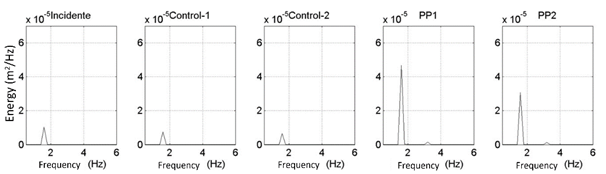
Figure 18 Energy spectra of the focalized wave for different depths and for different eccentricities obtained for each depth. The spectrum of the incident wave and control-1 and control-2 corresponding to tests PP1 and PP2, respectively, are shown.
The amplified energy for the case of PP1 was 4 times and 6 times with respect to the incident energy and the control point, respectively. For the case of PP2, it was 4 and 3 times with respect to the concentrated energy with respect to the incident energy and the control point, respectively, indicating that despite maintaining the eccentricity defined by the law of conic refraction, there is an important impact when the depth to which the lens is submerged is decreased, since for depths of the order of 1/3
Tests of change in the direction of the incident wave
Three tests were performed corresponding to angles of incidence with respect to the optical axis of 10°, 20° and 30°. To simulate the change in the angle of incidence, the elliptical lens was turned 10°, 20° and 30° clockwise. For each case, the instantaneous maximum free surface was graphed and the corresponding energy spectra were obtained at the point of maximum amplification.
Table 5 shows the cases evaluated where the angle of incidence and the position of the maximum are specified in x, y coordinates. Each test was given the acronym LED denoting Elliptical Lens Direction.
Table 5 Position of the focus generated for the direction tests. The average quadratic height obtained in the focus in coordinate pairs and the angle of incidence of the wave with respect to the optical axis is shown.
| Test | Angle | Focus position (X,Y) |
|---|---|---|
| LED1 | 10° | (3.68,2.44) |
| LED2 | 20º | (3.68,2.44) |
| LED3 | 30º | (3.72,2.44) |
Figure 19 shows the position of the focus for each of the cases evaluated, where the optical axis is indicated so as to have a reference of the change of position.
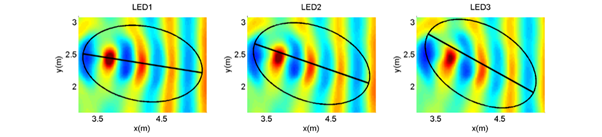
Figure 19 Maximum instantaneous free surface for 10° (ELD1, left panel), 20° (LED2, middle panel) and 30° (LED3, right panel).
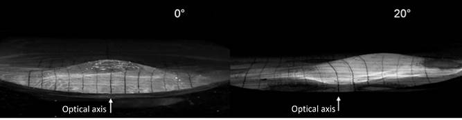
Figure 20 shows the spectra obtained at the positions indicated in Table 5, as well as the spectrum of the incident wave and at the control point. It can be observed in Figure 19 that as the angle of incidence of the waves increases, the focus moves to one side of the optical axis and the amount of energy concentrated by the lens decreases, from 5-6 times, and to 4 times and 6-7 times and 5 times the energy obtained at the control point, for LED1, LED2 and LED3, respectively (see Figure 20). The change of the position of the focus with respect to the optical axis was recorded by high-speed video in the FI-UNAM for the case of an angle of incidence of 20° (corresponding to LED2) and the displacement of the focal area coincides with the that was simulated with the CELERIS model (Figure 21).
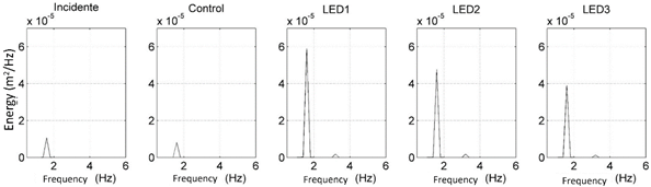
Figure 20 Focused wave energy spectra for different angles of wave incidence (10° LED1, 20° LED2 and 30° LED3). The spectrum of the incident and control waves is shown.
Conclusions
In this research the ability of submerged elliptical lenses to amplify wave energy that could be harnessed as a source of renewable energy was evaluated through numerical simulations with a Boussinesq type model. The CELERIS model was satisfactorily validated by means of laboratory tests in the FI-UNAM, showing that it is capable of simulating the focalization process adequately for waves with normal incidence and those with oblique incidence. With respect to the performance evaluation tests, it was found that with the geometries defined from the refractive index and/or the resulting eccentricity of the conics refractive law, the greatest amount of energy was obtained in the focal point, where the energy calculated obtained was between 7 and 8 times that at the control point. However, it was found that there are certain limits of water depth, installation depth and size of the respective semi-axes to
This article establishes optimal ranges for the design of a submerged elliptical lens from the incident wavelength, with which an energy concentration can be obtained which is approximately 8 times greater (during stable conditions) than without a submerged lens (point of control). In addition, lens performance metrics for different geometries are suggested, in terms of eccentricity and height, as well as depth of installation, thereby offering different alternatives.
Acknowledgements
For the financing of the development of this project, the CONACyT is thanked. Conacyt-Sener Fund (project ICCEO-232986) were responsible for partial financing, during the numerical simulations of the CELERIS model. The authors wish to thank Ing. Ponciano Trinidad Ramírez for support in the laboratory testing.
REFERENCES
Baquerizo, A. (1995). Reflexión del oleaje en playas. Métodos de evaluación y predicción (tesis doctoral). Santander, España: Departamento de Ciencias y Técnicas del Agua y del Medio Ambiente, Universidad de Cantabria. [ Links ]
Briganti, R., Musumeci, R. E., Bellotti, G., Brocchini, M., & Foti, E. (2004). Boussinesq modeling of breaking waves: Description of turbulence. Journal of Geophysical Research, 109, C07015, 1-17. [ Links ]
Cotter, C. D., & Chakrabarti, K. S., (1994). Comparison of wave reflection equations with wave-tank data. Journal of Waterway, Port, Coastal, and Ocean Engineering, 102(2), 226-232. [ Links ]
Dean, R. G., & Dalrymple, R. A. (1984). Water wave mechanics for engineers and scientists. New York, USA: Prentice-Hall. [ Links ]
Fuhrman, D. R., Bingham, H. B., & Madsen, P. A. (2005). Nonlinear wave-structure interactions with a high-order Boussinesq model. Coastal Engineering, 52(8), 655-672. [ Links ]
Griffiths, L. S., & Porter, R. (2011). Focusing of surface waves by variable bathymetry. Applied Ocean Research, 34, 150-163. [ Links ]
Kirby, J. T. (2003). Boussinesq models and applications to nearshore wave propagation, surf zone processes and wave-induced currents. Elsevier Oceanography Series, 67, 1-41. [ Links ]
Madsen, P. A., & Sorensen, O. R. (1992). A new form of the Boussinesq equations with improved linear dispersion characteristics. Part 2: A slowly-varying bathymetry. Coastal Engineering, 18, 183-204. [ Links ]
Mansard, E. P. D., & Funke, E. R. (1980). The measurement of incident and reflected spectra using a least squares method. Procedures (pp. 154-172). 17th Conference onCoastal Engineering , Sydney, Australia. [ Links ]
Mehlum, E., & Stamnes, J. (1978). On the focusing of ocean swells and its significance in power production (pp. 1-38) (SI Rep. 77). Bliundern, Oslo, Norway: Central Institute for Industrial Research. [ Links ]
Murashige, S., & Kinoshita, T. (1992). An ideal wave focusing lens and its shape. Applied Ocean Research, 14, 275-90. [ Links ]
Nwogu, O. (1993). Alternative form of boussinesq equations for nearshore wave propagation. Journal of Waterway, Port, Coastal and Ocean Engineering, 119(6), 618-638. [ Links ]
Prinos, P., Avgeris, I., & Karambas, T. (2005). Low-crested structures: Boussinesq modeling of waves propagation. Environmentally Friendly Coastal Protection. NATO Science Series. Series IV: Earth and Environmental Series, 53. Dordrecht, The Netherlands: Springer. [ Links ]
Soares, G. C., & Mohapatra, C. S. (2015). Wave forces on a floating structure over flat bottom based on Boussinesq formulation. Renewable Energies Offshore. London, UK: Taylor and Francis Group. [ Links ]
Stamnes, J. J., Lovhaugen, O., Spjelkavik, B., Chiang, C. M. L. E., & Yue, D. K. P. (1983). Nonlinear focusing of surface waves by a lens - theory and experiment. Journal of Fluid Mechanics, 135, 71-94. [ Links ]
Tavakkol, S., & Lynett, P. (2017). Celeris: A GPU-accelerated open source software with a boussinesq-type wave solver for real-time interactive simulation and visualization. Computer Physics Communications, 217, 117-127. [ Links ]
Received: January 15, 2018; Accepted: May 27, 2019
 Este es un artículo publicado en acceso abierto bajo una licencia Creative Commons
