Generalities

The hydrological design in the stages of planning, construction, operation and revision of hydraulic works, is based on the so-called Flood Design (CD, for its Spanish initials). That is in the case of reservoirs, protective levees, canals, bridges and/or urban drainage structures. CDs are maximum river flows associated with low probabilities of exceedance, whose most reliable estimate is made by means of the Flood Frequency Analysis (AFC), when hydrometric data of maximum annual flows are available.

The AFC is a probabilistic procedure consisting of the following five steps: (1) verification of the statistical quality of the data or available sample; (2) selection of a probability distribution function (FDP), or probabilistic model from which the data is likely to come, (3) estimation of the FDP fitting parameters; (4) calculation of predictions or values associated with a certain probability of non-exceedance, it is made based on the FDP tested and (5) selection of results, in an objective way, the best fit achieved with each FDP and method of estimating its parameters is sought (^{Kite, 1977}; ^{Stedinger, Vogel, & Foufoula-Georgiou, 1993}; ^{Rao & Hamed, 2000}; ^{Meylan, Favre & Musy, 2012}; ^{Salas, Obeysekera & Vogel, 2018}).

When there are no hydrometric data, the estimation of the CD is addressed through the so-called hydrological methods, which transform design hietograms into hydrographs or peak flow sought (^{Majumdar & Kumar, 2012}). Estimation of the design storms is based on the curves Intensity-Duration-Frequency, but due to the scarcity of pluviographic or rain-gauge records, it is usually done through the probabilistic analysis of rainfall records of maximum daily precipitation (PMD). These records are usually wider and have much higher spatial coverage (^{Teegavarapu, 2012}; ^{Johnson & Sharma, 2017}).

The AFC is identical to the probabilistic analysis of PMD records and therefore, the first step of both procedures is to verify that the annual data samples of maximum flows or PMD have been generated by a stationary random process, that is, that has not changed over time. This means that the record to be processed must not have deterministic components such as trend, persistence, or abrupt changes in the mean.

Unfortunately, the effects of global or regional climate change and the physical alterations suffered by the drainage basins or the surroundings of rain-gauge stations give rise to records of floods and of PMD that are nonstationary because they show trends. In general, the upward trends in the samples of floods are a consequence of urbanization or deforestation and the downward ones of the construction of reservoirs of use and/or control. In the series of annual PMD trends are commonly associated with the effects of regional climate change (^{Nguyen, El Outayek, Lim & Nguyen, 2017}; ^{Serago & Vogel, 2018}; ^{Salas et al., 2018}).

^{Khaliq, Ouarda, Ondo, Gachon and Bobée (2006)} concisely describe the various existing approaches to carry out the processing of non-stationary records. On the other hand, ^{El Adlouni, Ouarda, Zhang, Roy and Bobée (2007)} expose a specific procedure based on the fitting of the Generalized Extreme Values (GVE) distribution by means of the generalized maximum likelihood method and compare the stationary model (GVE₀) with the non-stationary that accepts linear dependence in its location parameter (u) with a covariate or GVE₁ model. When the dependence is quadratic or curve, the GVE₂ model is defined and when there is a linear dependence also in the scale parameter (α) the GVE₁₁ model is established. ^{El Adlouni and Ouarda (2008)} present the generalization of the L-moment method to the fitting of the non-stationary GVE₁ and GVE₂ distributions.

The previous approaches, as well as that of ^{Aissaoui-Fqayeh, El Adlouni, Ouarda and St. Hilaire (2009)}, allow the use of a covariate different from time, for example, those associated with global climatic behavior. ^{Campos-Aranda (2018)} presents examples of the application of the GVE₁ and GVE₂ models, using the generalization of the L-moments method and as covariates the time and the Southern Oscillation Index (SOI).

^{Serago and Vogel (2018)} suggest performing the probabilistic analysis of the non-stationary records, by means of a bivariate regression, which describes the relationship between the data (x) and the exogenous variable or covariate. Then they obtain the conditional mean, variance and asymmetry of x and y = ln (x), to apply them to the FDPs of three fitting parameters: Log-Normal (LN3), Log-Pearson type III (LP3) and stationary GVE and obtain their respective non-stationary models. The Log-Normal distribution was the first to reach a generalized application in the AFC, in the decade of the 1960s. LP3 and GVE functions were the first whose application was established under precept in the U.S.A. and England. GVE model became the classic distribution of the frequency analyses of hydrological extreme values and the LP3 function is the basic model of the AFC, therefore its non-stationary version (LP3₁), now developed by ^{Serago and Vogel (2018)}, will certainly have great significance in the estimation of CDs, through records with trending.

^{Salas et al. (2018)} indicate that ^{Serenaldi and Kilsby (2015)}, among other authors, have recommended that stationarity always remain as an option to apply in the AFC. This is justified by the fact that the non-stationary condition detected may not be caused by physical causes of anthropogenic actions or climate change, but may have been caused by low-frequency components of the ocean-atmosphere system ^{López-de-la-Cruz & Francés, 2014}; ^{Álvarez-Olguín & Escalante-Sandoval, 2016}) or by the effects of persistence (^{Khaliq et al., 2006}).

Objective

This study describes in detail the operating procedure of ^{Serago and Vogel (2018)}, to apply the stationary LN3, LP3 and GVE distributions and the non-stationary distributions LN3₁, LP3₁ and GVE₁ to records of floods and annual PMD showing linear trend. Two numerical applications are presented, the first to a record of 77 annual maximum flows and the second to a series of annual PMD with 58 data; both show an upward trend. The selection among the three FDPs is made based on the standard error of fit. The major contribution of this study is to describe and apply the non-stationary version of the LP3 distribution, applicable to records with trend, with a fairly simple method that corrects its quantile function.

Linear regression model

The general regression model, whose structure and theoretical properties will be analyzed and applied is (^{Serago & Vogel, 2018}; ^{Salas et al., 2018}):

in which, x are the data of the series of annual extreme hydrological values (floods, winds, levels, precipitations, temperatures, etc.), f(·) is a transformation of x to make it linear, w ₁ and w ₂ are the covariates of the climate or the land use, β ₁ and β ₂ are the coefficients of the model and ε is the model error, which is considered independent, with uniform variance and with Normal distribution.

^{Vogel, Yaindl and Walter (2011)} and ^{Prosdocimi, Kjeldsen and Svensson (2014)} have found that the previous model, when y = ln(x) and w ₁ is considered the time (t) in years, it is useful to analyze trending floods in U.S.A. and U.K. rivers, regardless of whether the trend was significant or not. ^{Serago and Vogel (2018)} emphasize that such a simple model does not imply any hypothesis regarding the FDP of the variable y. Besides, they modify the linear regression to introduce the mean values (μ) of the variables, and then we have:

now, the variable y is conditioned by the explicative variable w, β is the coefficient of regression and ε is once again the error of the model with mean zero and variance constant and equal to:

where, ρ is the linear correlation coefficient between y and w. Considering that there are no missing values in the annual series of extreme hydrological values and that their size is n, then the estimates in Equation (2) are (^{Prosdocimi et al., 2014}; ^{Serago & Vogel, 2018}):

whereby:

Applying Equations (6) and (7) to the original data x, their mean (x-) and standard deviation (σ _x ) are defined. Their asymmetry coefficient is calculated with the expression:

Non-conditional moments

According to ^{Serago and Vogel (2018)}, when performing a stationary frequency analysis, the moments of x and y = ln(x) do not depend on the explanatory variable w, therefore, they are non-conditional moments and are defined by their means (μ _x , μ _y ), standard deviations (σ _x , σ _y ) and asymmetry coefficients (γ _x , γ _y ).

Conditional moments of y

^{Serago y Vogel (2018)} use Equation (2) to obtain the conditional moments that will be used in the non-stationary frequency analysis, without making any consideration about the FDP of the variable y. The mean of Equation (2) leads to the expression of the expected value of y conditioned by w, this is:

Similarly, the conditional variance of y is obtained using Equations (3) and (10), to obtain:

The above equation shows that the conditional variance of y decreases as the explanatory power of the trend increases, tending to zero when ρ approaches the unit. On the contrary, when p tends to zero the conditional variance tends to the original. In general, in the non-stationary frequencies analysis the conditional variance of y is lower than the non-conditional variance. ^{Serago and Vogel (2018)} find that the conditional asymmetry of y is:

The above expression indicates that the conditional asymmetry of y is equal to the non-conditional asymmetry, when the asymmetry of the explanatory variable (γ _w ) is zero, case of w equal to time (t).

Conditional moments of x

^{Serago and Vogel (2018)} apply the exponential function to Equation (2) and obtain the expression:

in which, x _w and y _w are the conditioned values by the explanatory variable w. Note that hypothesis regard the FDP of x _w and y _w have not been established; but according to Equation (15) it is probable that x _w comes from a distribution Normal and that y _w does it from a Log-Normal function. The above is valid because the only variable on the right side of Equation (15) is the error of model ε and exp(ε), which are approximately Normal and Log-Normal, respectively.

To obtain the expressions of the conditional moments of x, it will be accepted that x _w approaches a Log-Normal distribution and then the equations that relate the mean, variance and asymmetry of x and of y =ln(x) are used in the Log-Normal distribution, which are (^{Serago & Vogel, 2018}):

Finally, Equations (16) to (18) are extended by applying expressions (12) and (13), to obtain:

Stationary LN3 distribution

If a series of annual extreme hydrological values (y) defined as y = ln(x - a) follows a Normal distribution with mean and standard deviation equal to μ _y and σ _y , then the variable x has a Log-Normal distribution of three fitting parameters (LN3), being a its lower limit or location parameter. Predictions associated with a certain return period (Tr), which is the reciprocal of the exceedance probability, are estimated with the expressions (^{Kite, 1977}; ^{Rao & Hamed, 2000}):

where:

being:

and:

In the above expression, γ _x is calculated with Equation (11). Finally, Z in Equation (23) is the standardized normal variable; it is estimated based on the following algorithm (^{Zelen & Severo, 1972}) for a non-exceedance probability (p):

with

c ₀ = 2.515517c ₁ = 0.802853c ₂ = 0.010328

d ₁ = 1.432788d ₂ = 0.189269d ₃ = 0.001308

this when 0 < p < 0.50, to do Z = -Z; in case that 0.50 < p < 1.0 use: p = 1 - p in Equation (29), without change Z.

Non-stationary LN3 distribution

The quantile function of the Log-Normal distribution of three non-stationary fitting parameters (LN3₁) is similar to Equation (23), but it uses conditional moments and variables (^{Serago & Vigel, 2018}):

To quantify axw with Equation (24), Equations (20) and (21) are used and to evaluate μxw by means of expression (25) the Equation (21) is used. In Equation (31), σ _y is defined with the expression (26), due to the fact that is only a function of γ _x (remember Equation (14)).

Stationary LP3 distribution

If a series of annual extreme hydrological values (y) defined as y = ln (x) follows a Pearson type III distribution, also known as a three parameter Gamma, then variable x has a Log-Pearson type III distribution (LP3). Predictions associated with a certain return period (Tr), which is the reciprocal of the exceedance probability, are estimated with the expressions (^{WRC, 1977}; ^{Kite, 1977}; ^{Bobée & Ashkar, 1991}):

and

In Equation (32), K _p is the so-called frequency factor, it is a standardized Pearson type III variable whose approximation is achieved based on the standardized normal variable Z (Equations (29) and (30)) and the corrected asymmetry coefficient (γ _c ), with the following equations (^{Kite, 1977}):

being:

and

Non-stationary LP3 distribution

Equation (33) is actually the quantile function of the LP3 distribution, whose non-stationary version (LP3₁) is obtained by substituting the conditional moments of y (Equations (12) and (13)), that is (^{Serago & Vogel, 2018}):

The constant values of the previous expression, from left to right, are defined in Equations: (6), (9), (4), (34), (7), (9) and (5), these last three, squared. For the calculation of K _p with the Equation (34), ^{Serago and Vogel (2018)} establish a different expression to Equation (35) for the asymmetry coefficient and define it as follows:

Stationary GVE Distribution

The Generalized Extreme Values (GVE) distribution includes three families of functions: the Gumbel that are straight lines on the Gumbel-Powell probability paper (^{Chow, 1964}), the Fréchet that are curves with upward concavity and lower limit, and the Weibull that have downward concavity and upper limit. Its quantile function is the following:

in which, u, α and k are the location, scale and shape parameters and p is the probability of non-exceedance. ^{Bhunya, Jain, Ojha y Agarwal (2007)} have proposed expressions to estimate the fitting parameters of the GVE, based on the mean (x-), standard deviation (σx) and coefficient of asymmetry (Yx), that is, based on the non-conditional moments; these are: when -0.70 ≤ γ _x ≤ 1.15

and when γ _x ≥ 1.15

for -0.50 ≤k ≤ 0.50, we have:

when 0.010 ≤ k ≤ 0.50

and when -0.50 ≤ k ≤ 0.010, the following Equation (44) is applied:

The values of x- and σ _x are obtained with Equations (6) and (7), using x instead of y. ^{Serago and Vogel (2018)} use Equation (11) to estimate the coefficient of asymmetry (γ _x ).

Non-stationary GVE Distribution

When equations of the conditional moments of x are applied, defined by Equations (20), (21), (22), and (19), in Equations (40) to (44), the fitting parameters of GVE distribution the non-stationary (GVE₁) are obtained, and they are named:uxw, axw and kxw, whose quantile function is (^{Serago & Vogel, 2018}):

Standard error of fit

The standard error of fit (EEA) has been established as a quantitative objective indicator, because it evaluates the standard deviation of the differences between the observed values and those estimated with the FDP that is tested; in this study the models: LN3, LP3, GVE, LN3₁, LP3₁ and GVE₁. Its expression is the following (^{Kite, 1977}):

in which, n and np are the number of data and of fitting parameters, in this case three, for the stationary FDP and four for the non-stationary ones; X _i are the data ordered from least to highest and X^i are the values estimated with the stationary quantile function (Equations (23), (33), and (39)) and non-stationary (Equations (31), (37), and (45)), for a probability of non-exceedance estimated with the Blom formulas for the models LN3, LN3₁, LP3 and LP3₁ and of Gringorten for the GVE and GVE₁ distributions, as suggested by ^{Serago and Vogel (2018)}:

where, m is the order number of the datum, with 1 for the least and n for the highest.

Approach of the probabilistic analysis

The EEA helps to select, among different distributions applied to the data or sample available, the one of better fit. Logically, such models must be of same type, stationary or non-stationary. Then, in each record to be processed, the LN3 and LN3₁ distributions are applied first, then the LP3 and LP3₁ and finally, the GVE and GVE₁; their EEA values are analyzed and the predictions sought are adopted. In this process, when the EEAs are similar, a distribution can be adopted based on hydrological safety judgments, that is, the one that reports the most unfavorable or critical predictions.

By means of Equations (31), (37) and (45) predictions are calculated with return periods (Tr) of 2, 25, 50 and 100 years, through the record period, applying the variable w _i in the interval from 1 to n. The first prediction is the median, since its probability of non-exceedance (F) is 50% and the following three are calculated for complementary probabilities, to define its higher and lower value (^{Park, Kang, Lee, & Kim, 2011}), that is, for the following values: F = 0.96 and F = 0.04 for the Tr of 25 years; F = 0.98 and F = 0.02 for the Tr of 50 years and F = 0.99 and F = 0.01 for the Tr of 100 years.

Predictions that use the variable w _i equal to the size of the record (n) correspond to the end of the historical record. Future predictions are possible using as magnitude of the variable w _i , the sum of the size of the record (n) plus the lapse in years to the future. Extrapolations of the predictions were made in three future dates, 10, 25 and 50 years after the available record is concluded.

^{Mudersbach and Jensen (2010)} establish that the hydrological design of hydraulic works must be reliable or safe until the end of its useful life or future date. If the record of floods or annual PMD available to estimate the CDs, shows an upward trend, then their predictions should be estimated at such future date so that their hydrological sizing is correct and not unsafe.

In this context, ^{Salas et al. (2018)} have suggested shortening the useful life values to 25 or 50 years and at the same time making the design and construction of hydraulic works more versatile, so that they allow for extensions and/or modifications at lower costs for society.

Records to be processed

The first series of extreme hydrological data corresponds to the annual maximum flows of the Neponset River in Norwood, Massachusetts, U.S.A., in the period from 1939 to 2015 (n = 77). This drainage basin has 89.8 km², with 16% of its extension of impermeable area, which has increased its maximum flows, but it is also a river with small reservoirs for municipal and industrial supplies (^{Serago & Vogel, 2018}). The approximate values read from a logarithmic figure of these authors are shown in Table 1 and Figure 1; it is observed that such record shows slight upward trend.

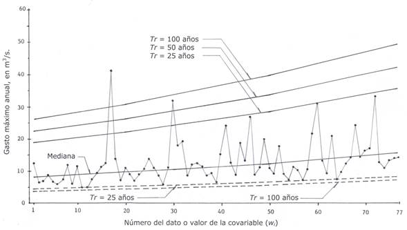
Figure 1 Chronological data series and estimated prediction curves with the LP3₁ distribution in a hydrometric station of the Neponset River, USA. 

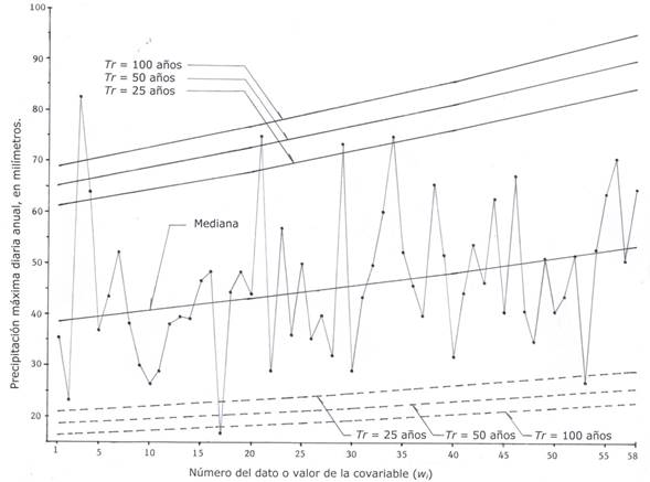
La second series of extreme hydrological data that was analyzed, comes from ^{Campos-Aranda (2016)} and corresponds to the annual maximum daily precipitations (PMD) ) of the Zacatecas climatological station, in the city of the same name in Mexico, with a record of 58 years in the period from 1953 to 2010. The series has an upward trend, as shown in Figure 2.

Figure 2 Chronological series of the annual maximum daily precipitation and estimated prediction curves with the LP3₁ distribution in the Zacatecas climatological station, Mexico. 

Predictions in the Neponset River

Table 2 shows a selection of the predictions obtained during the historical record with the LN3₁ distribution. The basic parameters of this non-stationary fitting were: ρ = 0.414, β = 0.0085, axw=3.807, uxw=2.4830, γc=1.83614 and σy=0.5182. Table 3 shows the EEA and the predictions of the stationary LN3 model with a = 0.5879 and μy=2.3842 and of the non-stationary, logically at the end of the historical record (n) and in the three future scenarios proposed.

Table 4 shows a portion of the predictions obtained during the historical record with the LP3₁ distribution. The basic parameters of this non-stationary fitting were: y-=2.4543 and σy=0.4569, ρ = 0.414, β = 0.0085 and γc = 0.53338. Table 5 shows the EEA and the predictions of the stationary LP3 model with γc = 0.53878 and of the non-stationary, at the end of the historical record (n) and in the three future dates analyzed.

Table 6 shows a part of predictions during the historical record, estimated with the GVE₁ distribution, with γxw=2.2731 and parameters of fit: uxw=14.015, axw =4.742 and kxw=-0.139. On the other hand, Table 7 shows the EEA and the predictions of the stationary GVE model with γ _x = 1.8361, u = 9.817, α = 4.607 and k = -0.101, as well as the non-stationary at the end of record and in the future in the three dates proposed.

Based on the values of the EEA shown in Tables 3, 5 and 7, the predictions or results of LP3 and LP3₁ distributions are adopted, against those of the LN3 and LN3₁, GVE and GVE₁ models, because they lead to their lowest magnitudes, indicating with it, a better fitting for the available data. Predictions of the non-stationary LP3₁ distribution were found to be the most severe or critical, thus providing greater safety in the hydrological design at the end of the useful life of 10, 25 or 50 years.

Figure 1 shows the chronological series of the Neponset River floods, U.S.A. and their estimated prediction curves with the non-stationary LP3₁ distribution.

Predictions in the Zacatecas station

Table 8 shows a part of the predictions obtained during the historical record with the LN3₁ distribution. The basic non-stationary parameters of fit were: ρ = 0.298, β = 0.0057, axw=-66.8647, μxw=4.7920,γ _c = 0.42827 and σy=0.1411. Table 9 shows the EEA and predictions of the stationary LN3 model with a = -54.6459 and μ _y = 4.6091 and of the non-stationary, logically at the end of the historical record (n) and in the three future scenarios proposed.

Table 10 shows a portion of the estimated predictions during the historical record with the LP3₁ distribution. The basic parameters of this non-stationary fitting were: y-=3.7962, σy=0.3218 , ρ = 0.298, β = 0.0057 and γ _c = -0.50869. Table 11 shows the EEA and the predictions of the stationary LP3 model with γc = -0.51495 and of the non-stationary at the end of the record and in the three future dates analyzed.

Table 12 shows part of the predictions during the historical record, estimated with the GVE₁ distribution, with Yx|w=2.1646 and fitting parameters: uxw=46.955, axw=10.950 and kxw=-0.131. In contrast, Table 13 show the EEA and the predictions of the stationary GVE model with γ _x = 0.4283, u = 40.896, α = 13.166 and k = 0.152, as well as the non-stationary, record term and in the three future dates proposed.

Based on the values of the EEA shown in Tables 9, 11 and 13 the predictions or results of the GVE and LP3₁ models are adopted, because they lead to their lowest magnitudes, thus indicating a better fitting to the available data. The predictions of the three stationary models are almost identical. The GVE₁ function reports more extreme or critical predictions, but its EEA is more than the double obtained with the LP3₁ distribution; therefore they were not selected.

Figure 2 shows the chronological series of annual PMD of the Zacatecas climatological station, Mexico and its straight lines of estimated predictions with non-stationary LP3₁ distribution.