


 texto en
  Inglés (pdf)
 Artículo en XML
 Referencias del artículo
 Enviar artículo por email
 Citado por SciELO
  Similares en
SciELO
Similares en
SciELO 
 Permalink
Introduction
One of the most frequently encountered cases of rapidly varied flow is the hydraulic jump phenomenon. The most important application of the hydraulic jump is in the dissipation of energy below spillways, weirs, gates, etc. Based on 3-D observations during experimental tests, the flow phenomena significantly differs from the classical hydraulic jump in trapezoidal and rectangular channels. The most extensively studied case of the hydraulic jump is in horizontal rectangular channels and detailed metric discussion. The schematic sketch of a typical hydraulic jump in a horizontal channel is depicted by Figure 1. The hydraulic jump and its steadiness in the trapezoidal channel are especially important. Scholars, such as Wanoschek and Hager (1989) and Muhsun (2012) analyzed the properties of trapezoidal channels through experimental tests. Hager (1992) and Chanson (2007) studied the undular hydraulic jump, and they described its characteristics where the values of the Froude number in which the jump is no longer than undular was calculated regardless of the effect of the channel width. Afzal and Bushra (2002) studied structure of turbulent hydraulic jump in trapezoidal channel.

The surface profile approaches as limiting universal solution provided that the variables are appropriately non-dimensionalized. Gupta, Mehta and Dwivedi (2013) investigated relative length and relative energy loss of free hydraulic jump in prismatic channels. Ohtsu (1976) classified the hydraulic jumps in trapezoidal channels into four types. The criterion involved the symmetry of the main current. Ohtsu (1976) recommended that only hydraulic jumps of types 1 and 2 ("the jump is almost symmetric") should be used as the energy dissipater. Kim, Choi, Park and Byeon (2015) has investigated hydraulic jump properties and it's energy dissipation in downstream with sluice gate. Javan and Eghbalzadeh (2013) has studied submerged hydraulic jump with k-ɛ turbulent modeling. Nezu et al. (1985) after studying the effect of roughness on experimental results in rectangular canal, even when boundary roughness conditions change, showed that the main structure of secondary currents does not change dramatically. Yaaghoubi and Givechi (2007) investigated the effect of secondary currents in the average velocity of cross sections in rectangular channels. After studying the effect of roughness on experimental results in rectangular channel, even when boundary roughness conditions change, the main structure of secondary currents does not change dramatically. Nezu, Nakagawa and Tominaga (1985), and Qin, Shao and Zhou (2016) made a comparison between two different secondary current correction moles for depth-averaged flow of meandering channels. Investigation of the distribution of boundary shear stresses in prismatic trapezoidal channels has also been studied by other researchers, including Dasgupta and Tomar (2015). Shokrian-Hajibehzad and Shafai-Bejestan (2017) predicted sequent depth ratio in hydraulic jump on river and the sequent depth ratio on rough rocky beds was found to be considerably smaller than those on a smooth concrete bed. Two new prediction equations, for smooth and rough bed slopes, are presented and the results showed that the predictions agree reasonably well with the experimental data.
Jalili-Ghazizadeh, Attari and Farhadi-Rad (2017) studied the hydraulic jump alongside weirs. In the model, the lateral outflow momentum is considered in which the model predicts the location of the hydraulic jump. Present study seeks to fill the research gap related to the investigation of secondary current cells in trapezoidal channels and their effect on hydraulic jump phenomenon which should be considered as the novelty of the research.
The present paper pursues two main objectives, including 1) the characteristics and properties of secondary currents in hydraulic jump for trapezoidal channels incorporating three various side slope angles (lateral angles) using both experimental and numerical approaches and 2) variation in energy loss in hydraulic jump relative to changes in Froude numbers for both experimental and numerical analyses, as well as comparison with findings obtained by Hager (1992). The main focus of the study is concentrated on different trapezoidal sections subjected to various flows discharge.
Secondary current cells
Generally, secondary currents are a subset of flows in the cross sections or around the axis perpendicular to the cross section of the flow. The currents in curves are called strong secondary currents, but those in prismatic channels of the plan are called weakly secondary currents. Secondary currents and open channels are significantly important in hydraulic engineering, due to the immense effect of these currents on the flow field, the impact of the friction rule and the formation of three-dimensional shapes on the beds of the channels.
Secondary currents equations
The main purpose for making secondary currents in a uniform longitudinal flow is the uniformity of the Reynolds stress disparity and, essentially, its vertical components. Prandtl (1904) dictated the two main mechanisms leads to rotational flows in the flow direction, namely, 1-deviation of the main shear stresses by a lateral pressure gradient or physical force, and 2-inconsistency and fluctuating turbulence in a plate perpendicular to the rotation axis. The longitudinal rotational equation in the fully developed turbulent flow is subrogated (Azhdari-Moghaddam, Tajnasaj, & Givech, 2013):
Where W and V refers to velocity components in horizontal direction (Z), and velocity components in vertical direction (Y), respectively.
In fact, these are the same secondary current components; where ϑ is kinematic
viscosity of fluid,
Figure 2 illustrates the difference of vertical stresses in the main structure of the secondary flows.

Figure 2 Non-dimensional lines
In the present work, variables Z and Y are in the order of X for velocity perpendicular to the flow axis and Z for velocity perpendicular to the channel bed. The following equation shows the hydraulic jump phenomenon in the current study as investigated based on the definition of rotational flows, so that curl is function in flow opposite to zero:
Where
Flow-3D modeling
Solving the CFD (Computational Fluid Dynamic ) problem usually consists of four main components: geometry and grid generation, physical model set up, solution and the post-process of the computed data. The set problem is computed to generate the geometry and grid, and the data are acquired in a well-known manner. The modeling of a phenomenon involves complex problems which can be resolved by developing a simple model. Therefore, while an ideal model should introduce the minimum amount of complexity into the modeling equations, it is important to be as accurate as possible. To conduct a numerical model of the secondary currents, initially, it is necessary to develop a numerical model of the mean velocity indifferent sections for obtaining the limits of a velocity change in a proper manners.
According to Bayon, Valero, García-Bartual and López-Jiménez (2016) the boundary value for the quantities KT and ɛT are usually assumed to determine the local equilibrium between the processes of production and decay of turbulent shear stress and a rule of wall velocity profile. In this research, the RNG (Renormalization Group) model was used due to its statistical methods for deriving average equations for disturbance quantities such as kinetic energy and its loss rate making it the best turbulence model for simulating a hydraulic jump. The flow-3D software is employed to obtain an accurate correlation between the solution and the convergence of responses, which are based on the geometric spectral flow and flow characteristics (Microsoft Corporation, 2015).
ADV signal correlation
Extensive explanations on ADV (Acoustic Doppler Velocimeter) principles of operation can be found in Nortek Operational Manual (Nortek-AS, 2013). The velocities are estimated by using a technique called a pulse coherent Doppler processing, where the ADV measures the change in phase of the return signal from two successive acoustic pulses. The acoustic return is not a reflection from a single target, but a superposition of the reflections from many individual particles contained in the sampling volume. A phase coherency is achieved if all particles in the sampling volume maintain their relative positions concerning each other, in which case the strength and relative phases of individual reflections would not change from one pulse to the next. However, Doppler noise is an inherent part of Doppler-based volume backscatter systems, and there are other sources of noise as well. Thus, the return signal from the second pulse is not a phase-shifted reproduction of the first pulse, but it contains a certain amount of noise, which can be added to the coherent part of the return signal (Nortek-AS, 2013):
Where S1’ and S2’ are the return signals from two adjacent pulses, S1 and S2 are the coherent parts of the signal, and N1 and N2 represent the random noise. In practice, the ADV estimates the phase shift between return signals from two successive pulses using a complex auto-correlation function, which has a phase and a magnitude. The phase is proportional to the distance which is traveled in the time between pulses by scatters, and thus to the velocity. The magnitude is a measure of how similar the echoes from two return signals are, and the normalized magnitude yields the correlation coefficient. If the echoes from two neighboring pulses were identical and only with a phase change, the correlation would be perfect and equal to 100%. As the echoes become more dissimilar, the correlation decreases. Low correlations are associated with highly turbulent flows, air bubbles in the flow, low SNR (Signal to Noise Ratio) values, large velocity gradients within the sampling volume, the presence of large individual particles, or interference from the boundary.
In turbulent flows such as hydraulic jump, it is reasonable to assume that the particles in the sample volume will not maintain their relative positions concerning each other, thus the Doppler noise of the return signal will be added. This will decorrelate the signal, and in this case low signal correlations will not necessarily mean that the data is undesirable. Also, if the turbulence eddies are of the same order as the sample volume or smaller, the correlation will change even more, which will lead to increase of the noise in velocity measurements. The correlation coefficient for turbulent flows will be discussed in more detail in the next section.
Experimental study
To create a hydraulic jump along the channel, several hydraulic modes have been tested in the laboratory model. Previous studies examined the classical jumps made for rectangular cross-sections. The experimental set-up and properties of channel are presented in Table 1.
Table 1 Geometric characteristics of channel.
| Type of channel | Length (m) | Width (m) | High of side wall (m) | Valve Opening (m) | Location of Valve (m) |
|---|---|---|---|---|---|
| m = 1.0 | 5 | 0.2 | 1 | 0.035 | 0.2 |
| m = 0.58 | |||||
| m = 0.26 |
Where m is the side slope of the channel and it is schematically represented in Figure 3. The numerical value of the side slope for angles 45°, 60° and 75° in this investigation was equal to 1.0, 0.58 and 0.26, respectively.

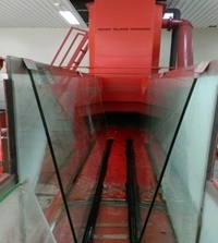
The volume of reservoir tank of beginning of the channel is 3.2 m3. Figure 4 and Figure 5 show Geometry characteristics of the channel and position of the ADV on the channel.
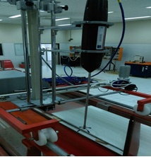
As shown in Figure 5, the ADV machine is mounted on a carriage, it moves on the channel using (Jog) software and sends the device to the designated depth at the desired location. In this paper, the measurements were carried out at 25 Hz for 2 minutes, with a total of 3000 impressions for the average point velocity (u, v, w).
Based on previous experience, the device is initially completely resting in laminar flow, so that the device can send the frequency inside the flow, then, lower discharge was used to harvest secondary velocities at the beginning of a hydraulic jump. The discharges used in this study were equal to 10, 30, 50, 70 and 90 lit/s, for three sectional geometry angles, including 45, 60 and 75° angles in trapezoidal channel.
The point that matters in Victorina+ software settings is that all values in the configuration of the trial and error must match in a coordinated manner obtained for all four recipients that the correlation coefficient must be greater than 70% and the SNR must be greater than 15dB (Martin, Fisher, Millar, & Quick, 2002). In the present study, the numerical value of SNR 23 dB to 24 dB is obtained.
It should be noted that the correlation coefficient is a parameter for determining the quality of the measurement of velocity in percent. In each measurement, the device calculates the correlation parameter for each audio receiver. The 100% correlation value at best indicates a low noise measurement and a zero correlation indicates the effect of noise reduction due to noise. Ideally, measurements should correlate 70% and 100%. Also, SNR is signal to noise ratio and the amount of this parameter in the measurements is indicative of the presence of sufficient particles in the water to disperse the sound. If the water is very clear and smooth, the return signal to the device receptors is weak, compared to the existing noise and the device will not be able to measure the velocity. During the measurement of turbulent flows such as hydraulic jumps, this ratio should not be lower than 15. In the present research, the pumps were used to determine the desired discharge in the channel. About Table 2, the state of pumps rpm is ready for realization of different discharges. It is worth noting that during the test, three pumps were utilized, in such a way that all other discharges were formed by combining two or three pumps, expect for the values of first two discharges.
Table 2 The status of the ultrasonic pumps
| Row | Type of pump | Round per minute (RPM) | Q (l/s) |
|---|---|---|---|
| 1 | Constant discharge | 1 754 | 33 |
| 2 | Variable discharge | 4 783 | 90 |
| 3 | 3 507 | 70 | |
| 4 | 2 659 | 50 | |
| 5 | 1 576 | 30 | |
| 6 | 896 | 10 |
The Vectrino device measures water velocity based on the Doppler phenomenon. Based on this phenomenon, if the audio source moves at v velocity to a sensitive receiver, the received audio frequency is calculated by the receiver according to the transmitter's audio velocity using the following equation:
Where FDoppler is changing frequency of the received sound and FSource is transmitter sound frequency; v is velocity of the transmitter to the receiver; c is sound velocity in fluid, which is assumed to be 1 484 m/s in the present study.
Figure 6 shows that how the device is placed inside the stream, which begins to flow at a discharge of 10 l/s to 90 l/s, and each discharge was taken for 2 minutes, and this discharge has been performed at all three angles of the channel.

In Figure 7, Figure 8 and Figure 9, the beginning of the hydraulic jump formed by the discharge of 90, 70 and 50 lit/s at 75° is shown.

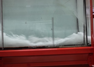
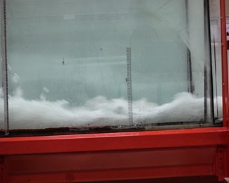
Table 3 and Table 4 present experimental and numerical results, respectively, and they illustrate five different discharges of 90, 70, 50, 30 and 10 l/s. These tables also present the Froude numbers before and after the jump, the initial depth, and ratio of the jump length to the secondary depth for all three geometric sections, which is done to show non-dimensional of the jump length.
Table 3 Experimental results in three Trapezoidal sections.
| m= 1.0 | m= 0.58 | m= 0.26 | ||||||||
|---|---|---|---|---|---|---|---|---|---|---|
| (Fr) |
|
Initial depth (m) | (Fr) |
|
Initial depth (m) | (Fr) |
|
Initial depth (m) | ||
| Q = 90 (l/s) | Before jump | 8.67 | 6.18 | 0.06 | 12.2 | 6 | 0.073 | 12 | 5.11 | 0.08 |
| After jump | 0.52 | 0.64 | 0.77 | |||||||
| Q = 70 (l/s) | Before jump | 7.79 | 6.13 | 0.05 | 7 | 5.9 | 0.057 | 4 | 6 | 0.062 |
| After jump | 0.73 | 0.76 | 0.84 | |||||||
| Q = 50 (l/s) | Before jump | 3.3 | 5.5 | 0.027 | 2.1 | 5.41 | 0.037 | 2.1 | 5.21 | 0.042 |
| After jump | 0.36 | 0.63 | 0.81 | |||||||
| Q = 30 (l/s) | Before jump | 2 | 4 | 0.024 | 1.86 | 4.9 | 0.03 | 1.1 | 4.7 | 0.038 |
| After jump | 0.28 | 0.31 | 0.38 | |||||||
| Q = 10 (l/s) | Before jump | 1.2 | 3.1 | 0.025 | 1.1 | 3.72 | 0.031 | 1.2 | 3.81 | 0.033 |
| After jump | 0.13 | 0.17 | 0.16 | |||||||
Table 4 Numerical results in three Trapezoidal sections.
| m= 1.0 | m= 0.58 | m= 0.26 | ||||||||
|---|---|---|---|---|---|---|---|---|---|---|
| (Fr) |
|
Initial depth (m) | (Fr) |
|
Initial depth (m) | (Fr) |
|
Initial depth (m) | ||
| Q = 90 (l/s) | Before jump | 9.72 | 6.92 | 0.05 | 10 | 6.83 | 0.055 | 9.2 | 6.18 | 0.071 |
| After jump | 0.73 | 0.87 | 0.87 | |||||||
| Q = 70 (l/s) | Before jump | 8.12 | 6.92 | 0.041 | 7.6 | 6.78 | 0.049 | 8.13 | 6.13 | 0.052 |
| After jump | 0.93 | 0.98 | 0.99 | |||||||
| Q = 50 (l/s) | Before jump | 5.39 | 6.74 | 0.031 | 7.31 | 5.35 | 0.036 | 7 | 5.5 | 0.043 |
| After jump | 0.97 | 0.59 | 0.33 | |||||||
| Q = 30 (l/s) | Before jump | 2.97 | 5.76 | 0.02 | 4 | 5.25 | 0.026 | 4.7 | 4 | 0.032 |
| After jump | 0.34 | 0.75 | 0.94 | |||||||
| Q = 10 (l/s) | Before jump | 2.48 | 4.9 | 0.021 | 2.62 | 4.4 | 0.033 | 3.76 | 3.1 | 0.039 |
| After jump | 0.2 | 0.93 | 0.5 | |||||||
Figure 10a and Figure 10b depicts the dispersion of SNR and correlation, respectively, in secondary currents in the direction of perpendicular to the flow axis (V x ) relative to the number of device impressions in the hydraulic jump. Figure 11a and Figure 11b, show the dispersion of SNR and Correlation in secondary currents in the direction of perpendicular to the flow axis (V z ) relative to the number of device impressions in the hydraulic jump. Concerning the Figure 10 and Figure 11, the correlation distribution at secondary currents velocities in the direction perpendicular to the axis (V x ) of flow was greater than the secondary velocities in the direction of the perpendicular to the channel bed (V z ). In high discharges, due to the higher flow velocity, the correlation mitigates in the direction perpendicular to the axis of flow (V x ).

Figure 10 (a) The process of data acquisition changes based on the time steps of the ADV frequency relative to the SNR in secondary currents in the direction V x ; (b) The process of data acquisition changes based on the time steps of the ADV frequency relative to the Signal Correlation in secondary currents in the direction V x .
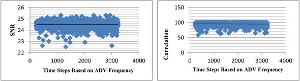
Figure 11 (a) The process of data acquisition changes based on the time steps of the ADV frequency relative to the SNR in secondary currents in the direction V z ; (b) The process of data acquisition changes based on the time steps of the ADV frequency relative to the Signal Correlation in secondary currents in the direction V z .
The velocity distribution trend in the horizontal direction (x) was higher in channels with less sidewall slopes, such as those with the 45° angle. The flow velocity is also higher in the horizontal direction (x) and therefore it leads to development of shear stress in the channels and eventually it reduces the hydraulic jump energy in the channel geometry, which in effect has a greater effect on higher discharges. In line with the objectives of this research and to investigate the secondary current cells in the horizontal direction (x), two high discharges, namely, 90 l/s and 70 lit/s were scrutinized. Discharges below these values do not dramatically affect the jump energy loss in secondary current cells within the horizontal direction (x). With increases in the flow velocity along channel (y), the velocity of secondary currents in x-direction increases more at 45° angle, compared to 60° and 75° angles.
In contrast, velocity vector distribution of secondary currents perpendicular to the flow surface (z) in the weaker discharge is greater than that of the side walls, due to the low flow velocity and the dominance of the gravity distribution velocity to the channel floor. This is the case in the velocity values of secondary flows in each of the three sections shown in Table 5 associated with experimental tests and Table 6 related to numerical modeling. As shown in Table 5 and Table 6, the velocity values are in the horizontal direction (x) for high discharges, and the values for the 45 and 60° angles section are in the vertical direction. Furthermore, velocity of the secondary currents in the vertical direction (z) for low discharges at 60 and 75° angles were greater than that of secondary currents in the horizontal direction (x).
Table 5 Experimental Secondary currents flow velocities in x and z direct.
| Row | Q (l/s) | m = 1.0 | m = 0.58 | m = 0.26 |
|---|---|---|---|---|
| 1 | 90 | V x = 0.36 m/s | V x = 0.31 m/s | V x = 0.26 m/s |
| V z = 0.22 m/s | V z = 0.25 m/s | V z = 0.27 m/s | ||
| 2 | 70 | V x = 0.33 m/s | V x = 0.18 m/s | V x = 0.15 m/s |
| V z = 0.26 m/s | V z = 0.29 m/s | V z = 0.49 m/s | ||
| 3 | 50 | V x = 0.21 m/s | V x = 0.16 m/s | V x = 0.11 m/s |
| V z = 0.39 m/s | V z = 0.5 m/s | V z = 0.6 m/s | ||
| 4 | 30 | V x = 0.14 m/s | V x = 0.1 m/s | V x = 0.07 m/s |
| V z = 0.41 m/s | V z = 0.52 m/s | V z = 0.81 m/s | ||
| 5 | 10 | V x = 0.11 m/s | V x = 0.05 m/s | V x = 0.01 m/s |
| V z = 0.49 m/s | V z = 0.61 m/s | V z = 0.92 m/s |
Table 6 Numerical Secondary currents flow velocities in x and z direct.
| Row | Q (l/s) | m = 1.0 | m = 0.58 | m = 0.26 |
|---|---|---|---|---|
| 1 | 90 | V x = 0.39 m/s | V x = 0.35 m/s | V x = 0.29 m/s |
| V z = 0.19 m/s | V z = 0.23 m/s | V z = 0.25 m/s | ||
| 2 | 70 | V x = 0.36 m/s | V x = 0.21 m/s | V x = 0.17 m/s |
| V z = 0.24 m/s | V z = 0.27 m/s | V z = 0.46 m/s | ||
| 3 | 50 | V x = 0.25 m/s | V x = 0.18 m/s | V x = 0.15 m/s |
| V z = 0.35 m/s | V z = 0.45 m/s | V z = 0.57 m/s | ||
| 4 | 30 | V x = 0.16 m/s | V x = 0.13 m/s | V x = 0.1 m/s |
| V z = 0.36 m/s | V z = 0.47 m/s | V z = 0.76 m/s | ||
| 5 | 10 | V x = 0.14 m/s | V x = 0.11 m/s | V x = 0.05 m/s |
| V z = 0.41 m/s | V z = 0.55 m/s | V z = 0.87 m/s |
Figure 12 illustrates variation in velocity of the secondary current in the direction of the vertical flow axis (V x ), which is plotted with changes in Froude numbers. Velocity of the secondary current cells for the cross-sectional of 45° angle in x-direction at different Froude number rates (Figure 12), was greater than the velocity of other sections in both experimental tests and numerical modeling. It can be concluded that the shear stress created in the side walls of this section is greater than the shear stress created in the other sections, which leads the flow towards the side walls. Figure 12 illustrates variation in the velocity of the secondary currents as shown in vertical direction (V z ) relative to the Froude number. The results show the trend to be opposite the horizontal (V x ) direction. Figure 13 illustrates changes in the velocity of the secondary currents, as shown in vertical direction (V z ) relative to the Froude number. The results show the trend to be opposite the horizontal (V x ) direction.

Figure 12 Comparison of secondary currents velocity in horizontal direct (V x ) with function of F1 for various m in Flow3-D and experimental tests.
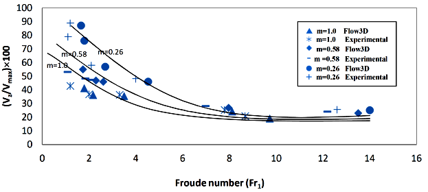
Figure 13 Comparison of secondary current velocity in vertical direction (V z ) with function of F1 for various m in Flow3-D and experimental tests.
According to the results of Figure 12, the equations governing the process of variation of the secondary currents velocity in the horizontal direction (Vx) versus the Froude number for each of the three sections follow the following relationships:
Moreover according to the results of Figure 13, the equations governing the process of variation of the secondary currents velocity in the vertical direction (Vz) versus the Froude number for each of the three sections follow the following relationships:
Velocity increases in horizontal directions when the cross-sectional changes from 75 to 45° angles in high Froude numbers. It is also possible to increase the vertical velocity (V z ) by changing the cross-sectional from 45 to 75° angles, in low Froude numbers. According to the data presented by Figure 12 and Figure 13, and Table 5 and Table 6, rough 33% and 28.9% growth rates can be obtained in a horizontal direction (V x ) of 75 ° to 60° angles in experimental tests, and in the same situation in numerical modeling, respectively, while about 44% at 60 to 45° angles in experimental tests and 32.6% in the same situation in numerical modeling can be obtained. Secondary velocity currents in vertical directions (V z ) were increased by 22.5% from 45 to 60° angles during experimental tests, while the currents were increased by 28% during numerical modeling, and they were increased by 42% from 60 to 75° angles during experimental tests. Moreover, the currents were increased by 47% during numerical modeling. The results of the data of Table 5 and Table 6 were compared using the root mean square error (RMSE) and determination coefficient (DC), which is calculated using following two relationships. The results are given in Table 7, and it can be deduced that, the maximum effect of secondary current velocity emerged in the horizontal direction (V x ) at 45° degree, and the maximum effect of secondary current velocity were in vertical direction (V z ) at 75° angle:
Table 7 Results of RMSE and DC for three geometry sections.
| V z | V x | |||
|---|---|---|---|---|
| Type of trapezoidal channel | DC | RMSE | DC | RMSE |
| m =1.0 | 0.77 | 0.098 | 0.91 | 0.067 |
| m =0.58 | 0.89 | 0.084 | 0.82 | 0.08 |
| m =0.26 | 0.95 | 0.08 | 0.85 | 0.07 |
The range of the DC is between 0 and 1 and as its value approaches toward 1, the situation gets the desirable. The value of the R.M.S.E is closer to the number 0 as it is. Therefore, the numbers 0.91 and 0.067 for the secondary currents velocity in the horizontal direction (V x ) and 0.95 and 0.08 for the secondary currents velocity in the vertical direction (V z ) are the best possible values for reaching to the desirable results. Figure 14 shows the sequent depths ratio Y2/Y1 as a functions of F1 for various (m) in both numerical modeling and experimental tests which was compared with the experimental results obtained by Hager (1992). Figure 15 illustrates comparison of hydraulic jump length L j /Y1 as a function of F1 for various (m) in present work and it was compared with the experimental results of Hager (1992). Figure 16 shows the variations of relative energy loss in a hydraulic jump. In Figure 16, the energy loss in the models performed is shown below the Froude number changes. It is evident that, in both numerical modeling and experimental tests the energy loss in trapezoidal sections with a lateral angle 45° angle was significant, compared to the other two sections with increasing Froude number. The obtained results were compared with that of Hager (1992) for better validation of the data for this energy loss chart in each of the three sections of this study.

Figure 14 Sequent depths ratio (Y2/Y1) as a functions of F1 for various m in Flow3-D and experimental tests.

Figure 15 The ratio of the hydraulic jump length to the initial depth (L j /Y1) as a function of F1 for various m in Flow3-D and experimental tests.

Figure 16 Comparison of relative energy loss in hydraulic jump as function of F1 for various m in Flow3-D models and experimental tests.
About Figure 15, the length of hydraulic jump in both numerical models and experimental tests at 45° angle has been increased with the increase in landing number, compared to the other two sections.
As shown in Figure 16, the energy loss in hydraulic jump at 45° angle cross section during experimental tests exhibited an increase of 4%, compared to Hager's results. Also, during numerical modeling at 45° angle, an increase of 9% in comparison with Hager’s results, was spotted. Generally speaking, these results indicate verification of the numerical and experimental tests. According to the comparison made between the results of numerical modeling and experimental tests, there is a desirable agreement between the results of these two models in all three geometric sections. So that, at 45° angle in the numerical models there is 5% increase compared to the experimental tests, and at 60° angle in the numerical models there is 11% increase compared to the experimental tests , and also at 75° angle in the numerical models there is 14% increase compared to the experimental tests. So that, the highest increase can be attributed to 45° section.
Conclusion
The boundary conditions used in this study are very effective in determining the boundaries of computations and sensitivities.
The velocity of secondary currents perpendicular to the axis of flow (V x ) in Froude number 10 of 45° angle is higher than the two other sections, which is 71% compared to 75° angle in numerical models and in Froude number 9 it was 91% in experimental tests.
The velocity of the secondary currents in the vertical direction of the flow surface (V z ) in Froude number 2 of 75° angle is higher than the two other sections, which is 88% compared to the 45° angle in numerical models and in Froude number 1.5 it was 74.5% in experimental tests.
The results demonstrated the existence of an inverse relationship between the velocity of the secondary current in the direction of the vertical axis of the flow (V x ) and the secondary velocity in the direction of the flow surface (V z ) during both numerical models and experimental tests.
Nomenclature
b |
is base width (m) |
Q |
is discharge (l/s) |
L j |
is length of hydraulic jump (m) |
W |
is velocity components in horizontal direction (m/s) |
V |
is velocity components in vertical direction (m/s) |
ϑ |
is kinematic viscosity (m2/s) |
denotes Reynolds normal stress (vertical) |
|
denotes Reynolds normal stress (horizontal) |
|
V x |
is velocity of secondary currents in horizontal direction (m/s) |
V z |
is velocity of secondary currents in vertical direction (m/s) |
is nebula operator |
|
i, j, k |
are unit coordinate vectors |
U |
is velocity in curl function |
is return signals from two adjacent pulses |
|
S1, S2 |
are coherent part of the signal |
N1, N2 |
are random noise |
m |
is cotangent of side slope |
Fr1 |
is Froude number before hydraulic jump |
Y2 |
is secondary depth of hydraulic jump (m) |
SNR |
is signal noise ratio |
Y2/Y1 |
is sequent depth ratio |
E1/ |
is relative energy loss of hydraulic jump |
RMSE |
is root-mean-square-error |
DC |
is determination coefficient |
c |
is velocity of sound (m/s) |
v |
is velocity of transmitter to the receiver (m/s) |
ψ |
is function of flow |
FDoppler |
is changing frequency of the received sound |
FSource |
is transmitter sound frequency |

