


 nueva página del texto (beta)
 Inglés (pdf)
 Artículo en XML
 Referencias del artículo
 Enviar artículo por email
 Citado por SciELO
  Similares en
SciELO
Similares en
SciELO 
 Permalink
Background
In Report No. 28 of the International Water Management Institute (IWMI), related with the evaluation of irrigated area in the Bhakra irrigation system in India (Sakthivadivel et al., 1997), using remote sensors and geographic information systems (GIS), a classification of the productivity of the land is made by using satellite images with which the values of the Normalized Difference Vegetation Index (NDVI) are calculated, and they are related with yields from the wheat crop, which dominates this irrigation system of 1.3 million hectares.
The basis of this evaluation is the relationship between the fraction of the photosynthetically active radiation and the crop’s yield. Indeed, this radiation called PAR describes the radiation available for the vegetation’s photosynthesis process. On the other hand, the fraction of solar radiation absorbed by the chlorophyll pigments (fPAR) describes the energy related with the assimilation of carbon dioxide and is derived from the PAR absorbed by the vegetative canopy, divided by the PAR available from sun radiation. It is assumed that fPAR is worth zero for the bare soil.
In this report, it is assumed that the photosynthetically active radiation absorbed by the crop (APAR) is related with the sum in time of the fPAR whose units are: (J m-2 t-1). It is also pointed out that APAR is the main parameter that controls the total biomass accumulated by the crop, so that the yield can be present as the following function:
Where Y is the grain yield in the crop and z is the
relationship between the grain yield and the total biomass, and
Then:
Where a and b are constants and NDVI is an expression directly linked with the crop’s yield. Based on this report, there is reference to several studies where the value of NDVI in anthesis (crop heading stage) is related, in order to estimate the crop’s yield, because in this stage an evaluation of the final yield of the crop can be made; in this regard, they mention the study by Pestamalci et al. (1995). However, in México a good linear relation was obtained between the yield in barley and the NDVI value in this stage of the crop’s development (Ruiz-Huanca et al., 2005).
For the case of wheat in India, the function found was the following:
With R2 = 0.8594 and standard error of 0.217 t/ha.
For the case of barley in México, the equation found was:
with R2 = 0.8846
In México also, a function for wheat in the south of the state of Sonora has been found, with a similar structure:
with R2 = 0.873 and standard error of 0.495 t/ha.
Materials and methods
The study research was performed in Irrigation District number 038, “Río Mayo”, in the south of the state of Sonora, located at coordinates -109.7873 W, 27.2912 N upper left corner and -109.2159 W and 26.7059 N lower right corner; it is irrigated with water from the “Adolfo Ruiz Cortínez” dam and 130 wells. The irrigable surface is 98,520 ha.
In this district, the geographic information system (GIS) is available with 15,022 plots detected, and it is divided into 16 irrigation modules, which are managed by 16 Water Users’ Associations (WUA) and a Limited Liability Society, which oversees the operation and maintenance of the infrastructure of the major network of canals, drainage and structures.
During the last four agricultural cycles, follow-up of the surface irrigated has been performed through monitoring with satellite images by Landsat 7, Landsat 8, and in a few months with Deimos 1 and RapidEye. To perform this monitoring, the NDVI (normalized difference vegetation index, Rouse et al., 1974) has been calculated, and the MSI (moisture stress index, Rock et al., 1986), using the corresponding reflectance calculated from satellite images, to which an atmospheric correction was applied and a multi-sensor normalization. In addition, the evapotranspiration of crops has been estimated as:
Where ETc is the crop’s evaporation and ETr is the evapotranspiration of reference, generally estimated through the Penman-Monteith equation, and the calculation of basal Kc as an empirical linear function of the NDVI (D’Urso and Calera, 2005, Calera et al., 2017).
The functions mentioned are:
Where: ρ i close infrared reflectance and ρ r reflectance in red
Where: ρ i close infrared reflectance and ρ im mid-infrared.
Coefficients of this function can vary depending on the crop; the values shown are valid for the wheat crop.

The average values of the indexes for each plot are estimated using a program developed by one of the authors of this article, and it calculates the average value of pixels plus fraction, within the limits of each GIS plot.
For the evaluation at the level of module or plot, modeling of the NDVI development (accumulated values) was carried out, assuming that this growth is proportional to the growth of the biomass and that it adjusts well to a sigmoid model, as J. H. Thornley (1976) suggests. Generally, between these models, those most frequently used are the Logistic and the Gompertz (Yin et al., 2003).
The differential equations on which the biomass development is based, for the case of the Logistic model, is
For the Gompertz model it is:
Where y is the dependent variable which, for this case, could be the amount of biomass, t the development time, k a constant of proportionality, and Y m the maximum value that the y variable reaches.
When integrating, the following functions are obtained:
Which can appear as
y0 is the initial value of the variable, which from (12) for t = 0 is worth:
For the Gompertz function it is:
Which usually appears as:
The growth rate is also usually used in both cases, based on functions (10) and (11); these rates that are presented as a bell function have a maximum value at the inflection point and are a good indicator of when the maturation and senescence of the crop begin. For the case of the Logistic function, the maximum value is reached at a time
For the case of the Gompertz function, this value is reached when
Specifically, for the case in consideration, it was seen that a better adjustment was achieved with the Logistic function, usually with values of the determination coefficient R2 higher than 0.99 and standard errors below 0.205 in the NDVI.
With regard to access to graphic satellite information by users of the Río Mayo irrigation district, they can enter the Web and see the state of their plots. First, they could access the information through the viewer generated in the PLEIADeS and SIRIUS projects, with servers in Spain, but since these projects are finished, another one was developed by “Colegio de Postgraduados” as part of a Master’s thesis, which is installed in the irrigation district of study.
Finally, in order to have another tool that allows performing an early estimation of yield, the heat units (Growing Degree Days: GDD) in Celsius degrees will be used, which allow evaluating the energy accumulated, from sowing to flowering, as well as the total accumulated until the end of maturation.
The climate information is obtained from INIFAP’s automatic station in the irrigation district’s center, for the whole period of crop development, daily, from October to May, by the state network of meteorological stations (Patronato para la Investigación y Experimentación Agrícola del Estado de Sonora) at: http://pieaes.dyndns.org/.
Results
During the last four agricultural cycles: 2011-2012, 2012-2013, 2013-2014 and 2014-2015, measurements were made of the wheat yield through sampling in several of the district’s irrigation modules, where this crop predominates, occupying between 75 % and 80 % of the module’s surface. In the first two cycles, a good relation was found between the maximum level of the NDVI and the average wheat yield; however, in the 2013-2014 cycle a small decrease was observed in the yield with regard to the expected one in agreement with function (5), but for the 2014-2015 agricultural cycle, the decrease in yield was highly significant, and the differences estimated in 6 of the modules evaluated varied between 20 % and 30 % less than in 2013-2014.
For the case of module 15, the estimation of the average wheat yield in the module was obtained through average value sampling of 6.91 t/ha in 2013, 6.62 t/ha in 2014 and 5.19 t/ha in 2015, a reduction of 1.72 t/ha equivalent almost to 25% of the yield obtained in 2013.
To understand the differences observed, the average NDVI values observed were graphed against the Heat Units: Growing Degree Days (°C) and the values for the maximum NDVI each year were also graphed against the yields as shown in Figure 2 (Parthasarathi et al., 2013).
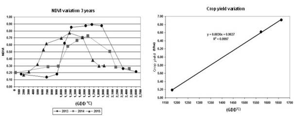
As complement to this figure, Table 1 shows a summary of the information that can be obtained with it.
Table 1 Information on Module 15
| Year | Max NDVI | GDD. total | Yield. t/ha | Max Day NDVI | GDD Max Val. |
|---|---|---|---|---|---|
| 2013 | 0.89 | 2331 | 6.91 | 128 | 1663 |
| 2014 | 0.73 | 2169 | 6.62 | 144 | 1573 |
| 2015 | 0.77 | 1809 | 5.19 | 96 | 1180 |
From Figure 2 and Table 1, it is deduced that the accumulation of Heat Units when the maximum value of the NDVI was present was reduced significantly in 2015 as compared to the prior years, and the same happens with the total HUs accumulated at the end of the crop, when the NDVI values reach a minimum of 0.3. These decreases imply that the crop did not accumulate enough energy to attain higher yields.
An analysis of the crop’s behavior was also performed in other modules where wheat is the predominant crop, Modules 5, 6, 10 and 13, whose results are shown summarized in Table 2 presented next.
Table 2 Information about the yield variation in 5 Modules.
| Module | Year | GDD at NDVI max | Total GDD | Yield t/ha | Yield dif. |
|---|---|---|---|---|---|
| Mod_05 | 2014 | 1573 | 2169 | 6.24 | |
| Mod_05 | 2015 | 1006 | 1678 | 4.81 | 1.43 |
| Mod_06 | 2014 | 1573 | 2463 | 6.51 | |
| Mod_06 | 2015 | 1180 | 1809 | 5.42 | 1.09 |
| Mod_10 | 2014 | 2046 | 2464 | 7.08 | |
| Mod_10 | 2015 | 1180 | 1921 | 5.19 | 1.89 |
| Mod_13 | 2014 | 1573 | 2464 | 6.83 | |
| Mod_13 | 2015 | 1180 | 1809 | 4.68 | 2.15 |
| Mod_15 | 2014 | 1573 | 2169 | 6.62 | |
| Mod_15 | 2015 | 1180 | 1809 | 5.19 | 1.43 |
As can be observed in this table, there was a significant reduction of the yields in every case, in all the irrigation Modules considered; in the case of Module 13, the reduction was almost a third of the yield obtained in 2014.
In general, there was a significant reduction of the Heat Units, which indicates a lower accumulation of energy in the crop, generating the yield reduction. To analyze the yield reduction in more detail, a more specific analysis for the case of Module 15 has been performed, where there is good information about the yields because the sampling was broader and more careful as a result of the participation of its directors who are producers that rent considerable surfaces.
For this case, modeling of the crop growth was performed, using the NDVI indexes accumulated, adjusting the variation to a sigmoid function of the Logistic type, and the rates of wheat crop growth were calculated for each one of the three years when their yields were available.
Adjustment of the values accumulated to a Logistic or Gompertz function was tested. The data were adjusted better to the Logistic model.
For 2013, the model:
For 2014, the model:
For 2015, the model:
In Figure 3, the curves generated with these functions have been graphed, showing that the longer the crop lasts, there was higher yield; it should be noted that in 2013, there was a longer duration of the crop than in 2015, and in 2014 it can be appreciated that there is an intermediate value.
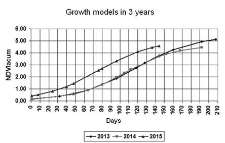
When calculating the growth rates of the wheat crop in these three years, it is observed that the values of the Heat Units for maximum NDVI value each year have differences, which are accentuated significantly between 2013 and 2015, as is shown in Figure 4, where in addition to graphing the rates with regard to the Hus, it has also been done in days. In both cases, the difference between 2013 and 2015 can be noted.

In the figures it can be seen that the growth rates in years 2013 and 2014 show certain similarities, with the variant of a higher maximum value in 2013; however, it is evident that the 2015 curve is completely out of phase, the maximum value happened prematurely, which agrees with the position of the NDVI values of the images shown in Figure 2.
The reason of the notable variation observed in the year 2015, among other variant meteorological conditions, was observed in this year, with many cloudy days, which probably generated a greenhouse effect, accelerating the development of the crop and preventing energy accumulation from happening, which is noted in the lower accumulation of HU.
When calculating the average evapotranspiration for module 15, it is observed that in spite of the differences in the crop’s development, the evapotranspiration in year 2013 was virtually equal to that in 2015, of around 390 mm, which implies that the daily evapotranspiration rate in 2015 was higher; this fact can also explain the greenhouse effect generated by cloudiness, which accelerated the crop’s growth.
Conclusions
It can be concluded that under “normal” meteorological conditions, an estimate of the yield value can be made based on the maximum NDVI value observed, which generally agrees with the time when anthesis happens, or flowering of the crop, as has been shown in the studies developed in different parts of the world, among which it can been seen in India and México.
However, a very fast growth of the biomass does not allow accumulating enough energy and, therefore, a decrease in yield can be expected, which could be proportional to the deviation observed in HU and even simply in days, with regard to the more frequent or “normal” value. Thus, an early estimation of the yield could be performed based on the maximum level of the NDVI, corrected in function of the date of its presentation, which allows evaluating the heat units accumulated.
Naturally, this work will require testing in other sites and possibly with more measurements to have a greater certainty about these conclusions. It is worth mentioning that there is more detailed information regarding the yield values in several plots, primarily in irrigation modules 13 and 15, with which a thesis study is being carried out to corroborate the prior results that are presented in this article.

