


Servicios Personalizados
Revista
Articulo
 texto en
  Inglés (pdf)
 Artículo en XML
 Referencias del artículo
 Enviar artículo por email
Indicadores
-
 Citado por SciELO
 -
 Accesos
Links relacionados
-
 Similares en
SciELO
Similares en
SciELO
Compartir

 Permalink
Tecnología y ciencias del agua
versión On-line ISSN 2007-2422
Tecnol. cienc. agua vol.10 no.1 Jiutepec ene./feb. 2019 Epub 21-Abr-2021
https://doi.org/10.24850/j-tyca-2019-01-06
Articles
Methodological procedure for a persistence drought monitor in Mexico
1Instituto Mexicano de Tecnología del Agua. Paseo Cuauhnáhuac 8532, Col. Progreso, Jiutepec, Morelos, CP 62550. rene_lobato@tlaloc.imta.mx
2Consultor en variabilidad, cambio climático y gestión del riesgo. Primera poniente 101, Isidro Fabela, Del. Tlalpan, Ciudad de México, CP 14030. mgaac@yahoo.com
3Facultad de Instrumentación, Electrónica y Ciencias Atmosféricas de la Universidad Veracruzana. Circuito Gonzalo Aguirre Beltrán s/n, Zona Universitaria, CP 91000. choyos@uv.mx.
4Instituto Mexicano de Tecnología del Agua. Paseo Cuauhnáhuac 8532, Col. Progreso, Jiutepec, Morelos, CP 62550. mario_lopezperez@tlaloc.imta.mx
5Instituto Mexicano de Tecnología del Agua. Paseo Cuauhnáhuac 8532, Col. Progreso, Jiutepec, Morelos, CP 62550. marco_salas@tlaloc.imta.mx
6Consultor independiente. jgperosario@gmail.com
An objective methodology for the detection and monitoring of droughts at a regional scale is presented. It is also shown how the drought monitoring can be detected and followed through the independent and joint index combination of the main hydrological (soil moisture), meteorological (precipitation and surface temperature), and vegetation (NDVI and evapotranspiration) indicators. The present methodology considers the information of each one of these variables, and additionally a joint estimation for precipitation and evapotranspiration is considered. Under this principle, it is proposed that the monitoring of droughts can be conducted through five indexes mainly, giving a different weight to each one depending of their spatio-temporal relevance. These indexes are standardized for an easy and practical combination following a weighted algebraic combination, derived from that an Index of Drought Persistence (IPS by its initials in Spanish) is obtained. The value of each one of the weights was determined in function of the relevance obtained through the principal components analysis; thus, it is obtained a single map, named persistence map, for each period considered ranging from one to 48 months. A comparative analysis with the actual and official Mexican Drought Monitor (MSM by its initials in Spanish) shows that the IPS is systematic, though it is complex to precisely determining how much due to the subjectivity that MSM is elaborated. Results from the IPS may be used as primary input for the water and agriculture sectors, but due to its nature and versatility, it is also possible to adapt the methodology to other users or sectors, including for climate change scenarios studies.
Keywords Drought; Drought Weighted Index; precipitation; soil moisture; principal components; drought persistence
Se presenta una metodología cuantitativa y replicable para el monitoreo (detección y seguimiento) de las sequías. Se demuestra que el monitoreo de las sequías se puede realizar, ya sea de una forma conjunta o independiente, mediante un número de índices que dependen fundamentalmente de variables meteorológicas (precipitación y temperatura superficial), hidrológicas (humedad del suelo) y de condición de la vegetación (NDVI y evapotranspiración). La presente propuesta metodológica considera información de cada una de estas variables, además de una estimación conjunta de precipitación y evapotranspiración. Con lo anterior, el seguimiento de la persistencia de la sequía se puede realizar con cinco índices fundamentales, dándoles una ponderación diferente en función de la importancia espacio-temporal. Estos índices son estandarizados de tal manera que sea fácil su combinación, derivando de ello un índice de persistencia de la sequía (IPS) a través de una integración algebraica ponderada. Se determinó el valor de la ponderación de cada índice en función de la importancia obtenida mediante un análisis de componentes principales. Así, se obtiene un solo mapa para cada período de tiempo considerado que va desde un mes hasta cuatro años (48 meses). El análisis comparativo con el actual Monitor de Sequías de México (MSM) elaborado por el Servicio Meteorológico Nacional (SMN) indica que el IPS por lo regular se aproxima en una categoría la intensidad de sequía aunque es complejo determinar la precisión del MSM debido a que su metodología contiene apreciaciones no cuantitativas. Los resultados del IPS demuestran su utilidad para los sectores hídrico y agrícola pero, por su flexibilidad, esta metodología se puede adaptar a otros sectores y, debido a su versatilidad, a estudios y proyección de escenarios de cambio climático.
Palabras clave sequía; índice ponderado de sequía; precipitación; humedad del suelo; componentes principales; persistencia de la sequía
Introduction
Drought is a recurrent natural phenomenon, with socio-environmental implications, which is part of climate variability; with intensity, variable spatial and temporal extension and that occurs in practically all climate regimes. According to Wilhite and Glantz (1987), the term of the drought has more than 150 different definitions depending on the sector that is affected and they are included in four basic categories depending on their temporality, magnitude and impacts; meteorological, agricultural, hydrological and socioeconomic.
The presence of droughts in Mexico is recurrent and irregularly spaced; it is a product of the climatic environment modulated by the forcing of hemispheric-type atmospheric patterns such as: El Niño Oscillation of the South (ENSO), the Decadal Oscillation of the Pacific (PDO), Atlantic Multidecadal Oscillation (AMO), among others (Florescano, 2000, Stahle et al., 2016).
Mexico is vulnerable to droughts, objective and quantitative results made through information extracted from tree rings describe that the first recorded drought was around the year 1400 (Stahle et al., 2016), better known as the drought of the "year one rabbit "where great havoc and a widespread famine caused death and long migrations to the survivors (Castorena et al., 1980).
Other sources of information obtained from codices and oral transmission, describe that drought occurred mainly during the years of 1004, 1064, 1286 and 1328 for the Valley of Mexico. It is very likely that a greater number of drought events occurred in other regions of the country, but unfortunately there is no information available; Florescano (2000) mentions that droughts have been present in the country since as early as 1500 BC.
Evidence suggests that drought events have increased in frequency, duration and intensity, especially in the tropics and subtropics, since the last half of the 20th century in response to global climate change (Zhang et al., 2007; Lynch et al., 2008; IPCC, 2012). In 2009, for example, it was considered the second worst drought in 60 years in Mexico that was experienced; and in 2011 the worst drought occurred in the last seven decades, covering approximately 80% of the Mexican territory with some degree of affectation (Figure 1), which resulted in large losses in sectors such as agriculture and livestock, affected mainly by water scarcity (Méndez, 2013), and an estimate in damages of 7,751 million pesos (approximately 700 USD million at 2011 prices) (CENAPRED, 2012).
As noted for its impacts, a change in hydrological systems, such as those caused by drought, imposes a significant risk to society (Jenkins and Warren, 2015), and even more so with the possibility of an increase in the frequency, severity and/or duration of the drought under climate change conditions. Therefore, it is urgent to understand the situation of current and future drought (Wang et al., 2015), which reinforces the need to plan for this phenomenon, given that small changes in the average climate can have significant impacts on water availability. (Bouma et al., 1996).
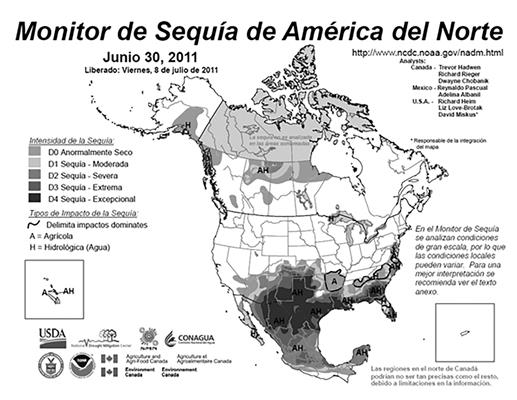
Figure 1 Available at: http://smn.cna.gob.mx/es/climatologia/monitor-de-sequia/monitor-de-sequia-de-america-del-norte
As part of efforts to understand, diagnose and monitor drought systematically and objectively, a series of indexes have been developed, taking as a quantitative measure derived from one or several meteorological, hydrological or other variables (indicators) that simplify the complex relationships between different climatic, hydrological parameters as: soil moisture, vegetation condition and others combined by various techniques (Tsakiris et al., 2007), that facilitate communicating information about climate anomalies to all types of audience, and also allow scientists to evaluate quantitatively the anomalies of the climate in terms of its intensity, duration, frequency and spatial extent (Méndez, 2013).
There are a number of indexes currently accepted and described by the World Meteorological Organization and the Global Water Partnership (WMO & GWP) (2016) where they are grouped by the type of indicator: Meteorological (23), Hydrological ( 4), soil moisture (8), vegetation (10), combined or modeled (5).
There are two categories of drought indices (Wang et al., 2015). The first contains multi-scale indices based on the characterization of humidity and dryness; for example, the Standardized Drought Index (SPI - McKee et al., 1993), the Standardized Index of Precipitation and Evapotranspiration (SPEI - Vicente-Serrano et al. 2010), the Standardized Soil moisture Index (SSI - Hao and AghaKouchak, 2013; Mo and Lettenmaier, 2014) or the Standardized Runoff Index (SRI - Shukla and Wood, 2008; Mo and Lettenmaier, 2014). The second category includes drought indices generated with bucket models of one or more layers, for example, Palmer's Drought Severity Index (PDSI, Palmer, 1965), Palmer's Moisture Anomaly Index (Z index; Palmer, 1965) or the Palmer Drought Severity Autocalibrated Index (sc-PDSI; Wells et al., 2004).
Some other indices, for example those derived from remote sensors (Zargar et al., 2011; Choi et al., 2013), have shown good performance in several countries, for example the normalized difference vegetation index (NDVI) provides good correlations, except under conditions of limited energy balance during the growth of vegetation in the cold season and at high latitudes (Anderson et al., 2013).
However, drought studies focus on changes of one or two of their characteristics, such as frequency or duration (Weiβ et al., 2007; Lehner et al., 2006; Burke et al., 2006; Hirabayashi et al., 2008; Blenkinsop and Fowler, 2007) while omitting other features that in parallel could contribute to a robust global assessment of drought trends and be useful for assessing economic and social consequences. For example, Steila (1987) points out that studies have shown that the humidity situation of a region is constituted by more than just the precipitation received, while McEvoy et al. (2012) showed that the inclusion of an additional term (temperature) of water demand, through the SPEI, could improve the information to represent the variability of hydrological drought in arid regions. In this way, and because multifactorial aspects affect the drought, it is not advisable to use a single index to monitor all its attributes (Keyantash and Dracup, 2002).
Having seen the above in a conceptual model of water balance, it is true that atmospheric pressure (convergence and divergence of flow) and surface temperature condition the soil moisture content; that is, not only precipitation is a determining factor to measure the magnitude of droughts, it is the interaction ocean-atmosphere-soil-vegetation and finally human intervention that closes the water cycle and therefore the balance thereof.
Then defining the precipitation, temperature, soil moisture, vegetation condition (NDVI and evapotranspiration) as base indicators for more accurate monitoring of droughts, it is proposed to use the information of each one of these as standardized indices.
An important component in the present investigation is to weight objectively through the application of principal components analysis to conventional drought indices such as SPI, SPEI, together with remote sensing indices as the NDVI and complementary temperature indices and soil moisture to monitor the persistence of the drought in Mexico, in terms of 1, 3, 6, 9, 12, 24 up to 48 months.
The proposed drought persistence index (IPS) allows monitoring of the drought of the meteorological, agricultural and hydrological type, by diagnosing the phenomenon at different time scales. Thus, the Water and Agriculture Authority, as the scientific community and users in general can count on a complementary tool to monitor the drought.
Data and methods
Study area
The Mexican Republic is located in the American continent in the northern hemisphere, between the Atlantic and Pacific oceans (National Institute of Statistics and Geography (INEGI), 2014).
Mexico has a varied climate (Figure 2a) as it is in the transition between dry subtropical and tropical climates; it is a dry type in the northern region of the country and the Altiplano towards the center of the country, but here it becomes much colder due to the altitude. It is temperate from the center to the coasts to move to tropical climates towards the south of the country; and it is warm humid and sub-humid from the coastal area of the Gulf of Mexico and the Pacific to the southern border of Mexico and the Yucatan Peninsula. The precipitation regime is monsoon with rainfall predominantly in the summer. While the distribution of the annual average precipitation (Figure 2b) is maximum in the south of the country, with values higher than 2,000 mm, and in the northwest and center north of the country the precipitation may even be less than the 400 mm.
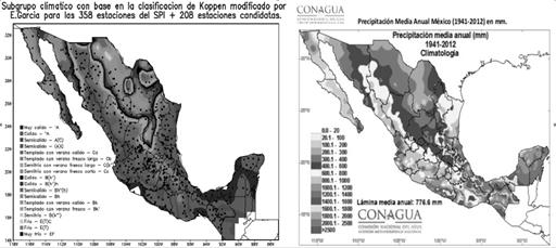
Figure 2 a) Climate according to the Köppen classification modified by García (1964). Source: IMTA; b) Mean annual rainfall. Source: SMN.
Data bases and methodology
To calculate a drought persistence index (IPS), it was considered to include the variables of precipitation, temperature, soil moisture and an index obtained by remote sensing, the NDVI; based on the importance of its signal in relation to the drought and recurrence in its use in research on drought indices. For the selection of the data bases of the selected parameters, the following criteria were considered: 1) that the data are aggregated monthly, 2) the spatial resolution of the data is 0.5 ° or finer, 3) the temporal extension of the data is older or equal to 15 years, 4) the temporality and availability of the data is at least one month out of phase with respect to the most recent current date for which the IPS is calculated. The detail of the availability of the database is shown in Table 1.
Table 1 Sources and characteristics of the data bases
| Parameter | Period | Resolution | Source | Format | |
|---|---|---|---|---|---|
| Spacial | Temporal | ||||
| rainfall | 1961-actual | Puntual | Daily | SMN/CLICOM | ASCII |
| Temperature | 1961-actual | Puntual | Daily | SMN/CLICOM | ASCII |
| NDVI | 2002-actual | 0.05° | Monthly | Land Processes Distributed Active Archive Center (LP DAAC) https://lpdaac.usgs.gov/dataset_discovery/modis/modis_products_table/mod13c2_v006 | HDF-EOS |
| Soil moisture | 1961-actual | 0.5° | Monthly | NOAA/Climate Prediction Center (CPC) | NetCDF |
The NDVI data were averaged in cells of a resolution of 0.5°, with the same geographic location as the rest of the databases. For the case of temperature, 354 points or sites of climatic stations distributed throughout the national territory were considered, which later on were interpolated to a 0.5° resolution grid using the Cressman method (1959) contained in the Grid Analysis and Display System (GrADS).
The referred databases were analyzed under a probabilistic approach to obtain indexes by parameter through the adjustment of probability distribution functions (FDP) to the series of each of the 12 months of the year. The PDFs were adjusted to the monthly accumulation of precipitation, soil moisture or precipitation-evapotranspiration and for temperature and NDVI were adjusted to the monthly average value, in the analysis periods of 1, 3, 6, 9, 12, 24 and 48 months.
The probability of the PDFs is transformed into a standardized normal dimensionless index, with zero mean (μ = 0) and unit standard deviation (σ = 1); positive values correspond to wet and negative to dry conditions, in order to be comparable and weights and objective combinations are made with them.
Precipitation
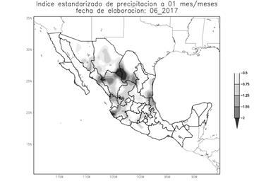
The multi-temporal SPI based on precipitation was used (McKee et al., 1993). The FDP Gamma of two parameters is adjusted to the precipitation series.
Where α> 0, shape parameter; β> 0, scale parameter; x> 0, precipitation of a certain period (1, 3, 6, 9, 12, 24 and 48 months); Γ (α), factorial mathematical function or gamma function (originally known as Pearson type III). Figure 3 shows a map where spatially represents the SPI on a 1-month scale.
Temperature
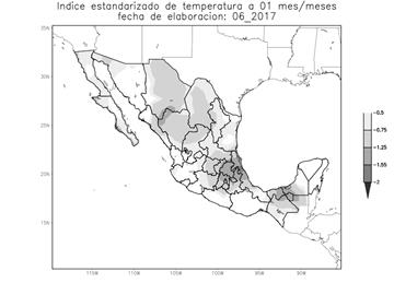
The Normal PDF was adjusted in a probabilistic analysis, based on the results of the Kolmogorov-Smirnov goodness test and the Chi-square test with respect to other PDFs such as Log-Normal, Weibull, Generalized Extreme Values and Gaussian Mixture. The Normal function is defined as:
With two distribution parameters: μ the average value and σ is the standard deviation (σ> 0), as well as a mathematical constant π with a value of 3.14159 ... Figure 4 shows a map where spatially represents the Standardized Temperature Index on a scale of 1 month.
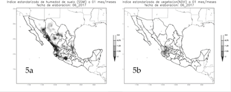
Soil moisture and NDVI
The Log-Normal FDP was adjusted in a probabilistic analysis, based on the results of the Kolmogorov-Smirnov kindness test and the Chi-square test with respect to other PDFs such as Normal, Generalized Extreme Values and Weibull. This distribution is frequently referenced in research on the environment (Castañeda et al., 2002). The Log-Normal distribution tends to the FDP:
where
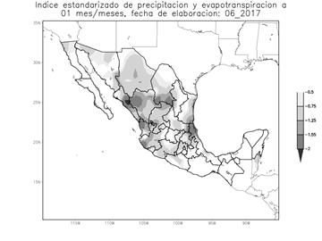
Precipitation-evapotranspiration
The SPEI precipitation-evapotranspiration index was implemented (Vicente-Serrano et al., 2010), applying the same algorithm and program proposed by the authors, which, based on rainfall, temperature and latitude data, obtains a water balance between precipitation and potential evapotranspiration (ETP) monthly, calculated with the formula of Thornthwaite (1948).
where
The water balance series is adjusted with the FDP of three parameters of the Log-Logistics distribution
where α, β and γ are the scale, shape and origin parameters. Figure 6 shows a map of the SPEI at a scale of 1 month with data until the month of June 2017.
Standardization of the índices
The cumulative probability of the PDFs, which define the indexes, is standardized based on the procedure defined for the SPI. According to Edwards and McKee (1997), a rational numerical approximation, presented in Zelen and Severo (1965), is used to convert the cumulative probability H (x) into the normalized standard variable Z, with μ = 0 and σ = 1
where
Allocation of weights
Initial weights were assigned to each index when evaluating the results of the principal component analysis (CP) applied to the series of each of the indices; this analysis identifies components (factors) that successively explain most of the total variance of a phenomenon with linear combinations of the original variables. In general terms, when inspecting the CP analysis of the total variance explained, the majority of the time lapses presented a similar behavior, so the representative period was taken as a 6-month period from 2002 to 2013, to consider a common period of analysis of the indices and neglect from the analysis data after 2013, that showed low information density for the temperature variable.
The recurrent order of the indices (temperature: STI, soil moisture: SSMI, SPEI, precipitation: SPI and SNDVI) that explain the highest variance is component one with a value of 52.4499% and component two with 22.5336% respectively, these eigenvalues can be visualized by means of a simple graph oriented to evaluate the relative importance of each one of the extracted principal components. Cattell (1966) proposed that this diagram could be used to determine graphically the optimal number of factors to be retained. Four components were generated (Figure 7) and the eigenvalues of component one indicate that there is a correlation in original indexes close to 0.5 in the SPI, SSMI, SPEI and SNDVI indices and a correlation close to zero (negative value) with the index STI, so with component one a linear combination was made. Observe in Figure 7 that the first eigenvalue captures 52.4499% of the variability of the data. However, this trend decreases as three other components are added to the model, which is, the decline is stabilized when considering the four main components.
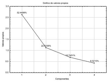
In this case, it was decided to retain the first two components since they explain 74.9835% of the variance. Jolliffe (2002) suggests that it can often be a reasonable range if it oscillates between 70% and 90% and allows a graphic representation in two dimensions and where there is also a change of slope in the graph (Wilks, 2006). Figure 8 shows the variability of the observations or marks on the axes formed by the first two main components, that is, the graphic representation of the matrix of components analyzed is displayed. The point-individual cloud is centered on the origin. The same does not occur with the cloud of variables in figure 7. The index points (SPEI, SPI, SNDVI and SSMI) can be all located on the same side, except the temperature index (STI). This is because the characteristics are positively correlated. It is observed that the coordinates of the index-points are lower in an absolute value of one. This is due to the fact that the indexes have been typified, with which their distance to the origin is one, and when projecting them on the axes, a contraction can be produced and to approach the origin, but never a distancing.
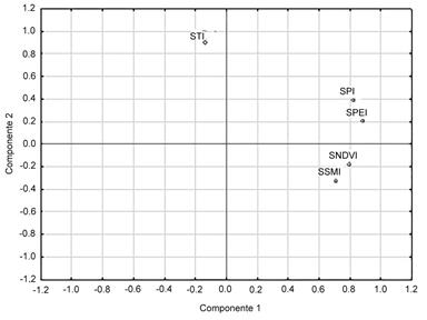
With the above, there are two groups formed, the first is a group where it is related in a certain way to water stress and which are opposed to the STI index, that is, the groups are formed as follows: group 1: SPEI, SPI, SNDVI and SSMI and group 2: STI.
In the first instance, greater weight was assigned to the indices that explain the greater amount of the total variance, identified in the CP. The weights were adjusted semi-iteratively, after a qualitative review of the drought maps of the IPS in each iteration with respect to maps of the SMN drought monitor, considered as a reference since they are the only ones of an official nature in the country. The monthly maps of the year 2008 (with low drought signal) and 2011 (with high drought signal) were compared based on the criterion of the least number of pixels without coincidence with drought data between the IPS maps and those of the SMN.
From the analyzes, it is found that the variable that has the greatest influence on the drought results is the soil moisture. The IPS finally proposed with its weights assigned to each index to calculate the drought using a linear combination is:
The drought classification of the IPS (Table 2) returns to the categories that are applied in the United States of America Drought Monitor (USDM, Svoboda et al., 2002), extended to the Drought Monitor of Mexico by the SMN ( Lobato-Sánchez, 2016).
Table 2 Drought classification used in the USDM (Svoboda et al., 2002)
| Category | Description |
|---|---|
| D0 | Anomalous dry |
| D1 | Moderate drought |
| D2 | Severe drought |
| D3 | Extreme drought |
| D4 | Exceptional drought |
The results of the IPS were evaluated with respect to those of the MSM through the application of conventional metrics, such as the mean, root mean square error (RMSE) and the Pearson correlation (Wilks, 2006).
Results
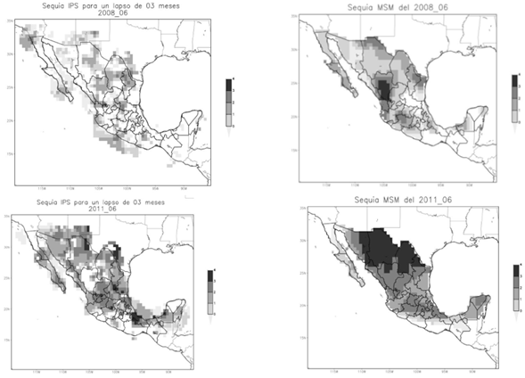
The ability of the IPS to represent the drought was analyzed when comparing the results with the one calculated by the SMN, the official source in the country for the generation of climate information through the Mexican Drought Monitor (MSM). The drought categories of both sources are comparable. The year 2008 was considered as a case study, with a low signal of drought, and the year 2011, considered as a year with high impact and economic damages due to the drought registered in Mexico (Figure 1 and 9).
Qualitatively, the IPS indicates greater spatial detail of the drought while the MSM indicates continuous polygons and of greater extension of the same one. The MSM drought, with category 3 and 4, is underestimated in the IPS in the center-west, in the extreme northeast and in the extreme north of the country in June 2008. The IPS partially captures the drought pattern of the MSM, of category 3 and 4, in the center of the country in June 2011; however, underestimates the drought in the areas of the northern portion and the Yucatan Peninsula and overestimates on the Baja California Peninsula.
The strength of the IPS is that it is an objective and measurable methodology. The difference in results compared with the MSM is systematic despite the methodologies of elaboration of each of them. This situation could be better adjusted with the calibration, as part of work to be developed, with respect to drought reports and their impacts in the field. A complement for validation purposes is the proposal for the development of an impact report at the national level, where users can feed back the IPS for a better accuracy of the phenomenon's condition.
For the objective analysis of the results, it was considered to apply conventional metrics (mean, standard deviation, mean square error, correlation) to the drought calculated with the IPS and the MSM, but given that the series of drought data of the MSM is short; As of 2007, it was found that the results (not presented) were not statistically significant.
The metric with robust results are tercils, calculated as
The difference of ranks/categories of drought was obtained for the cells in which the IPS indicates presence of drought. Tercils are classified as: Lower tercil considers differences less than -1; Neutral tercil is for differences between -1 and 1; and Upper tercil is for differences greater than 1.
It is found that the neutral tercil, with values usually above 60%, is the most recurrent condition of the difference between the drought calculated with the IPS with respect to that of the MSM (difference between both of ± 1 category of drought intensity) for lapses less than 12 months (Table 3 and 4, Figure 10), especially in the central-northern region of Mexico, followed by the intercalation of the overestimation tercil and the underestimation of the drought. While for periods greater than 12 months, the ability of the IPS is degraded, with percentages lower than 60% and even cases with a high percentage in the lower tercil (underestimation) are presented for the months with the highest drought intensity during 2011. In general terms, the tendency of the IPS in most of the country is to underestimate the drought reported by the MSM, while in the Peninsula of Baja California the IPS frequently overestimates the drought.
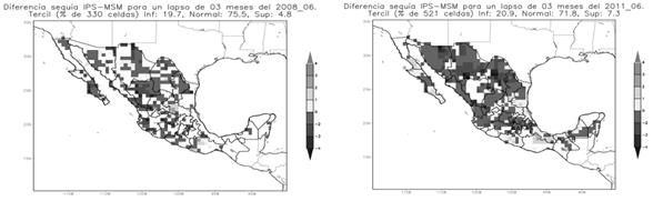
Figure 10 Tercil of the difference of the calculated drought with the IPS with respect to MSM for the month of June of years 2008 and 2011.
Table 3 Results of the neutral tercil (in %) for the months of 2008 for each drought time lapse.
| Lapse/month | 1 | 3 | 6 | 9 | 12 | 24 | 48 |
|---|---|---|---|---|---|---|---|
| 1 | 81.4 | 82.7 | 86.6 | 69.5 | 73.7 | 60.8 | 73.2 |
| 2 | 74.2 | 78.5 | 83.3 | 71.3 | 82.4 | 75.6 | 70.3 |
| 3 | 84.7 | 84.0 | 83.3 | 76.9 | 75.6 | 71.9 | 75.5 |
| 4 | 84.1 | 83.6 | 82.4 | 75.3 | 78.4 | 75.3 | 76.0 |
| 5 | 80.7 | 82.9 | 79.4 | 78.5 | 76.6 | 71.3 | 73.2 |
| 6 | 76.3 | 75.5 | 76.9 | 72.9 | 70.2 | 70.9 | 69.5 |
| 7 | 79.8 | 80.2 | 80.6 | 83.8 | 77.3 | 74.6 | 75.3 |
| 8 | 84.2 | 84.8 | 80.1 | 82.9 | 80.0 | 71.8 | 72.4 |
| 9 | 97.9 | 91.5 | 84.2 | 84.1 | 84.3 | 75.5 | 69.5 |
| 10 | 95.1 | 89.4 | 84.1 | 81.1 | 80.9 | 74.2 | 67.9 |
| 11 | 81.9 | 88.3 | 88.2 | 82.2 | 85.4 | 73.9 | 69.2 |
| 12 | 84.3 | 89.1 | 85.9 | 82.5 | 76.9 | 73.8 | 68.8 |
Table 4 Similar as above, corresponding to year 2011.
| Lapse/month | 1 | 3 | 6 | 9 | 12 | 24 | 48 |
|---|---|---|---|---|---|---|---|
| 1 | 61.8 | 60.9 | 72.8 | 77.2 | 87.9 | 74.7 | 80.7 |
| 2 | 60.4 | 61.0 | 69.0 | 71.2 | 81.7 | 75.6 | 80.3 |
| 3 | 72.8 | 60.7 | 55.6 | 63.9 | 69.9 | 66.3 | 65.9 |
| 4 | 75.7 | 74.5 | 65.8 | 48.7 | 53.5 | 57.2 | 58.0 |
| 5 | 80.9 | 81.4 | 74.5 | 60.3 | 48.0* | 50.8 | 56.5 |
| 6 | 77.2 | 71.8 | 65.7 | 59.2 | 51.5* | 54.1* | 52* |
| 7 | 78.3 | 83.4 | 74.6 | 67.7 | 54.2 | 53.8 | 55.8 |
| 8 | 76.9 | 80.2 | 78.2 | 73.9 | 65.6 | 58.7 | 61.1 |
| 9 | 76.8 | 75.1 | 71.6 | 66.9 | 64.4 | 62.9 | 57.7 |
| 10 | 78.9 | 81.2 | 82.3 | 80.7 | 73.4 | 57.0 | 49.2 |
| 11 | 85.4 | 80.6 | 80.7 | 77.4 | 71.2 | 58.8 | 48.8 |
| 12 | 84.0 | 81.8 | 79.6 | 76.8 | 73.1 | 59.1 | 52.4 |
* corresponding to the upper tercil.
The Mexican Institute of Water Technology (IMTA) updates monthly the IPS, thus generating a more representative statistical sample of maps of the persistence of drought in the country. Next, qualitative results are discussed when comparing the IPS maps with the MSM maps.
The IPS responds in a natural way to the spatial and temporal distribution of the observations or climatic and hydrological information with which its indices are elaborated separately. In principle, it is designed so that there is little or no human intervention, except to provide the corresponding information in each calculation cycle and for the interpretation of the results. The entire system depends on the calculation methodology as well as on the available information. Each one of the indices to elaborate the IPS has a different preponderant effect, the precipitation is reflected in the meteorological scale, but the soil moisture considers a longer temporal process, this is one reason why it is defined as a process with greater "memory". In our case and derived from the study carried out, is the humidity of the soil of greater importance to the rest of the considered indices.
It is complex to compare the spatial-temporal pattern because in one single map, the MSM tries to reflect the drought conditions and their impacts within the short, medium and long-term ranges; On the other hand, the IPS proposes to represent the evolution of the phenomenon for different time ranges within the same spatio-temporal scale.
The IPS shows that it is an effective tool to describe drought patterns under different ranges of time and space. The patterns are represented, although not precisely by the difference in methodologies, there is no way to determine the correct methodology because there are no checks that allow correction and subsequent calibration, it is observed the regions where there is some derivative effect not only because of the precipitation deficit, the effects of the other indicators are also considered.
Conclusions and recommendations
The developed tool of the IPS is appropriate for monitoring the persistence of the drought. Amono the strengths / advantages of the IPS are:
- It is a solid, objective and replicable methodology that dispenses with human intervention for its calculation.
- Represents in more detail the polygons of the drought compared to those of the MSM.
- The difference with respect to the MSM is systematic, which allows in the future making adjustments of linear type.
- It is a process that can be replicable or repeatable and obtain the same result, an important aspect within the scientific method.
It was evaluated, adjusted and standardized probability density functions (Gamma, Normal and Log-Normal, among others) to build indexes from historical series of precipitation, temperature, soil moisture and vegetation condition, based on good practices identified in drought indices applied nationally and internationally; constructed in probabilistic rather than deterministic form, for example the SPI and SPEI.
The indices generated in the study were assigned a factor to be weighted linearly in a global objective index; the IPS. The approach to the weights carried out, in the first instance, were based on the analysis of statistical parameters of the main components, with which the level of explanation of the indices to the total variance was characterized.
The ability of the IPS, represented in drought maps was analyzed with respect to the MSM. The tercile metric was applied to evaluate the ability of the IPS, since results from other metrics (mean, RMSE, correlation) were not robust for this purpose, due to the short period of the MSM drought series; as of 2007, in which episodes of drought and inter-drought are not well captured, which have occurred in previous years.
A relevant aspect to keep in mind is that the evaluation of the IPS's ability was performed with respect to the MSM, considered as official reference, which applies different procedures to calculate the drought by including a subjective evaluation to give differentiated and variable weights to the layers of information based on the experience of the climatologist.
The values of the IPS are close to those of the MSM since the neutral tercile is the most recurrent condition of the difference between the drought calculated with the IPS with respect to that of the MSM (difference between both of ± 1 category of drought intensity), with values greater than 60%, especially in the central-northern region of Mexico, followed by the intercalation of the overestimation tercile and the underestimation of the drought.
The use of different drought indices and the combination of remote sensors, such as the NDVI case, allowed a multifactor approach to climate adversity and its temporary visualization through specific illustrations (maps), so this new tool is proposed for quasi-real time monitoring of water conditions with emphasis on droughts, their assessment and diagnosis in the short and medium term. The timely identification of a drought will contribute, mainly, to the administration of the use of water resources reserves. However, the severity of the adverse effects generated by the drought requires the joint effort of the different spheres of government, universities, research centers, agricultural associations, finance agencies, insurance companies, and the society represented by the different users of water, as well as the deeper knowledge of the behavior of this phenomenon.
Based on the findings, it is recommended that in future investigations the IPS be strengthened when considering:
Calibration of the IPS based on reports of drought in the field.
Analyze the maps of each index, as well as the IPS in relation to La Niña, El Niño and Neutral events for future analysis given that the drought could be influenced by large-scale circulation patterns that are forced by low frequency variations of the sea surface temperature in the Pacific and Atlantic oceans.
Incorporate additional variables related to teleconnections, for example the sea surface temperature in the Pacific Ocean and ice cover in northern latitudes.
Support to interpret the results of the IPS with charts of surface winds and high and low pressure systems, this will help to identify dryness of the air that is reflected in a deficit of water vapor and / or in the alterations in the circulation of the winds.
Likewise, it is important to identify that, along with the improvement of the monitoring/monitoring systems of the drought, it is necessary to move towards the perspective of the drought, in the short and medium term, and the determination of the same, in the long term, under climate change scenarios for Mexico. In this sense, it is recommended to take up and materialize recommendations made by international organizations; for example NOAA (2007), where stressed the need to develop a new objective approach to predict drought that allows robust and transparent verification for users, and have sufficient flexibility to generate related probabilistic information through different time scales (monthly, seasonal, among others) to meet specific needs of decision making.
Finally, a system of early warning before the drought that contemplates the methodological analysis of the possible impacts under realistic scenarios can greatly help the official institutions, private initiative and users to act before the occurrence and therefore reduce the associated risks.
Referencias
Anderson, C. M., Hain, C., Otkin, J., Zhan, X., Mo, K., Svoboda, M., Wardlow, B., & Pimstein, A. (2013). An intercomparison of drought indicators based on thermal remote sensing and NLDAS-2 simulations with U.S. Drought Monitor Classifications. Journal of Hydrometeorology, V(14), 1035-1056. DOI: 10.1175/JHM-D-12-0140.1. [ Links ]
Blenkinsop, S. & Fowler, H. J. (2007). Changes in European drought characteristics projected by the PRUDENCE regional climate models. International Journal of Climatology, (27), 1595-1610. [ Links ]
Bouma, W. J., Pearman, G. J. & Manning, M. R. (1996). Greenhouse: Coping with Climate Change. Melbourne, Australia: CSIRO Publications. [ Links ]
Burke, E. J., Brown, S. J. & Christidis, N. (2006). Modeling the recent evolution of global drought and projections for the twenty-first century with the Hadley centre climate model. Journal of Hydrometeorology, (7), 1113-1125. [ Links ]
Castañeda, J. A., Gil, A., Jacky, F. & Pérez, A. (2002). Tamaño de muestra requerido para estimar la media aritmética de una distribución lognormal. Revista Colombiana de Estadística, junio, 31-41. [ Links ]
Castorena, G., Sánchez, M. E., Florescano, E., Padillo R. G. & Rodríguez V. L. (1980). Análisis histórico de las sequías en México: documentación del Plan Nacional Hidráulico. México: Secretaría de Agricultura y Recursos Hidráulicos. [ Links ]
Cattell, R. B. (1966). The Screen test for the number of factors. Multivariate Behavioral Research, 1(2), 245-276. [ Links ]
Cenapred. (2012). Características e impacto socioeconómico de los principales desastres ocurridos en la República Mexicana en el año 2011. (1a . ed.). Ciudad de México: Centro Nacional de Prevención de Desastres. [ Links ]
Choi, M., Jacobs, J. M., Anderson, M. C. & Bosch, D. D. (2013). Evaluation of drought indices via remotely sensed data with hydrological variables. Journal of Hydrology, (476), 265-273. [ Links ]
Cressman, G. P. (1959). An Operational Objective Analysis System. Monthly Weather Review, (87), 367-374. [ Links ]
Edwards, D. C., & McKee, T. B. (1997). Characteristics of 20th century drought in the United States at multiple time scales. Climatology Report, 2(97), Department of Atmospheric Science, Colorado State University, USA. [ Links ]
Florescano, E. (2000). Breve Historia de la Sequía (2ª ed.). México: Consejo Nacional Para la Cultura y las Artes. [ Links ]
García, E. (1964). Modificaciones al sistema de clasificación climática de Köppen. (3ª. ed.). México: Instituto de Geografía, Universidad Nacional Autónoma de México. [ Links ]
Hao, Z. & AghaKouchak, A. (2013). Multivariate Standardized Drought Index: A parametric multi-index model. Advances in Water Resources, (57), 12-18. DOI:10.1016/j.advwatres.2013.03.009. [ Links ]
Hirabayashi, Y., Kanae, S., Emori, S., Oki, T. & Kimoto, M. (2008). Global projections of changing risks of floods and droughts in a changing climate. Journal of Hydrological Sciences 53(4):754-772. [ Links ]
INEGI. (2014). Anuario Estadístico y Geográfico de los Estados Unidos Mexicanos 2013. Recuperado de: http://www.inegi.org.mx/prod_serv/contenidos/espanol/bvinegi/productos/integracion/pais/aeeum/2013/AEGEUM2013.pdf. [ Links ]
IPCC. (2012). Managing the risks of extreme events and disasters to advance climate change adaptation. A Special Report of Working Groups I and II of the Intergovernmental Panel on Climate Change. Cambridge, UK: Cambridge University Press. [ Links ]
Jenkins, K. & Warren, R. (2015). Quantifying the impact of climate change on drought regimes using the Standardized Precipitation Index. Theoretical & Applied Climatology. (120), 41-54. DOI 10.1007/s00704-014-1143-x. [ Links ]
Jolliffe, I. T. (2002). Principal Component Analysis (2a . ed.). United Etates: Springer-Verlag New York, Inc. [ Links ]
Keyantash, J. & Dracup, J. A. (2002). The quantification of drought: An evaluation of drought indices. Bulletin of the American Meteorological Society, (83), 1167-1180. [ Links ]
Lehner, B., Döll, P., Alcamo, J., Henrichs, T. & Kaspar, F. (2006). Estimating the impact of global change on flood and drought risks in Europe: a continental, integrated analysis. Climate Change, (75) 273-299. [ Links ]
Lobato-Sánchez, R. (2016) El Monitor de Sequías de México, Tecnología y ciencias del agua, 7(5), 197-212. [ Links ]
Lynch, A., Nicholls, N., Alexander, L. & Griggs, D. (2008). Defining the impacts of climate change on extreme events. Garnaut Climate Change Review, 1-19. [ Links ]
McEvoy, D. J., Huntington, J. L., Abatzoglou, J. T. & Edwards, L. M. (2012). An evaluation of multiscalar drought indices in Nevada and Eastern California. Earth Interactions, 16. DOI: 10.1175/2012EI000447.1. [ Links ]
McKee, T. B., Doeskin, N. J., & Kleist, J. (1993). The relationship of drought frequency and duration to time scales. In: Proceedings of the Eighth Conference on Applied Climatology. United States of America: American Meteorological Society. [ Links ]
Méndez, M. (2013). Diagnóstico y Pronóstico de Sequía en México. (informe OMM / MOMET-043). México: Comisión Nacional del Agua y Organización Meteorológica Mundial. [ Links ]
Mo, Kingtse C., y Lettenmaier, D. P. (2014). Objective drought classification using multiple land surface models. Journal of Hydrometeorology. American Meteorological Society. V 15. 990-1010. [ Links ]
NIDIS. (2007). The National Integrated Drought Information System implementation plan: A pathway for national resilience. 29 pp. Recuperado de http://www.drought.gov/imageserver/ NIDIS/content/whatisnidis/NIDIS-IPFinal-June07. [ Links ]
Palmer, W. C. (1965). Meteorological drought. Weather Bureau. Department of Commerce. Unite States of America, 58 pp. [ Links ]
Shukla, S., & A. Wood, W. (2008). Use of a standardized runoff index for characterizing hydrologic drought. Geophysical Reseach Letters, 35(2) L02405, DOI: 10.1029/2007GL032487. [ Links ]
Stahle, D. W., Cook, E. R., Burnette, D. J., Villanueva, J., Cerano, J., Burns, J. N., Griffin, D., Cook, B. I., Acuña, R., Torbenson, M. C. A., Sjezner, P. & Howard, I. M. (2016). The Mexican Drought Atlas: Tree-ring reconstructions of the soil moisture balance during the late pre-Hispanic, colonial, and modern eras, Quaternary Science Reviews, 149, 34-60. [ Links ]
Steila, D. (1987). Drought. En Olivier, J. E. & Fairbridge, R. W. (Eds.), The Encyclopedia of Climatology, New York: Van Nostrand Reinhold Company, pp. 388-395. [ Links ]
Svoboda, M., LeComte, D., Hayes, M., Heim, R., Gleason, K., Angel, J., Rippey, B., Tinker, R., Palecki, M., Stooksbury, D., Miskus, D., & Stephens, S. (2002). The Drought Monitor. Bulletin of the American Meteorological Society, 83(8):1181-1190. [ Links ]
Thornthwaite, C. W. (1948). An approach toward a rational classification of climate. Geographycal Review, (38), 55-94. [ Links ]
Tsakiris, G., Loukas, A., Pangalou, D., Vangelis, H., Tigkas, D., Rossi, G., & Cancelliere, A. (2007). Drought characterization. Chapter 7. Options Méditerranéennes, (58), 85-102. [ Links ]
Vicente-Serrano, S. M., Beguería, S. & López-Moreno, J. I. (2010). A Multi-scalar drought index sensitive to global warming: The Standardized Precipitation Evapotranspiration Index - SPEI. Journal of Climate, (23) 1696-1718. [ Links ]
Wang, H., Rogers, J. C., & D. Munroe, K. (2015). Commonly used drought indices as indicators of soil moisture in China. Journal of Hydrometeorology. American Meteorological Society. 16, 1397-1408. DOI: 10.1175/JHM-D-14-0076.1. [ Links ]
Weiβ, M., Flörke, M., Menzel, L. & Alcamo, J. (2007). Model-based scenarios of Mediterranean droughts. Advcanced Geoscienses. 12, 145-151. [ Links ]
Wells, N., Goddard, S. & Hayes, M. J. (2004). A self-calibrating Palmer drought severity index. -Climate, 17, 2335-2351, DOI: 10.1175/1520-0442(2004)017, 2335:ASPDSI.2.0.CO;2. [ Links ]
Wilhite, D. A. & Glantz, M. (1987). Chapter 2 Understanding the Drought Phenomenon: The Role of Definitions. En: Wilhite, D. A., Easterling, W. E. & Wood, D. A. (eds.), Planning for Drought: Toward a Reduction of Societal Vulnerability (pp. 11-27). Boulder, CO., United States of America: Westview Press. [ Links ]
Wilks, D. S. (2006). Statistical methods in the atmospheric sciences (2a . ed.). United States of America: Academic Press. [ Links ]
Organization (WMO) & Global Water Partnership (GWP), (2016). Handbook of Drought Indicators and Indices (Svoboda, M. & Fuchs, B.A.). Integrated Drought management Programme (IDMP), Integrated Drought Management Tools and Guidelines Series 2. Geneva. [ Links ]
Zargar, A., Sadiq, R., Naser, B. & Khan, F. I. (2011). A review of drought indices. Environmental Reviews, (19) 333-349. [ Links ]
Zelen, M. & Severo, N. C. (1965). Probability functions. In: Abramowitz, M., & Stegun, I. (eds.). Handbook of Mathematical Functions, 925-995. New York, U.S.A: Dover Publications. [ Links ]
Zhang, X., Zwiers, F. W., Hegerl, G. C., Lambert, F. H., Gillett, N. P., Solomon, S., Stott, P. A. & Nozawa, T. (2007). Detection of human influence on twentieth-century precipitation trends. Nature, 448(7152), 461-465. [ Links ]
Received: October 09, 2017; Accepted: June 26, 2018
 Este es un artículo publicado en acceso abierto bajo una licencia
Creative Commons
Este es un artículo publicado en acceso abierto bajo una licencia
Creative Commons
