


Servicios Personalizados
Revista
Articulo
 texto en
  Artículo en XML
 Referencias del artículo
 Enviar artículo por email
Indicadores
-
 Citado por SciELO
 -
 Accesos
Links relacionados
-
 Similares en
SciELO
Similares en
SciELO
Compartir

 Permalink
Tecnología y ciencias del agua
versión On-line ISSN 2007-2422
Tecnol. cienc. agua vol.9 no.5 Jiutepec sep./oct. 2018 Epub 24-Nov-2020
https://doi.org/10.24850/j-tyca-2018-05-11
Articles
Harmony search to optimize the univariate Gumbel Mixed Model

1 Centro de Investigaciones del Agua, División de Investigación y Posgrado Facultad de Ingeniería, Universidad Autónoma de Querétaro, Santiago de Querétaro, Querétaro, México, valnahar@hotmail.com
2 Centro de Investigaciones del Agua, División de Investigación y Posgrado Facultad de Ingeniería, Universidad Autónoma de Querétaro, Santiago de Querétaro, Querétaro, México, alfonso.gutierrez@uaq.mx,
3 División de Estudios de Postgrado de la Facultad de Ingeniería, Universidad Nacional Autónoma de México, Jiutepec, Morelos, México, francisco.aparicio@conagua.gob.mx
Phenomena analyzed in the field of engineering with frequency analyses are usually extreme events such as floods and droughts. Such events frequently have as origin the simultaneous occurrence of two phenomena, and therefore are analyzed with two simultaneous probability distributions. Such is the case of the climatological and hydrometric series in Mexico which, due to its exposure to phenomena such as hurricanes, are analyzed with two-population probability distributions. The good use of these distributions depends on the correct estimation of their parameters. The application of a harmonic search meta-heuristic algorithm for the estimation of the parameters that optimize the univariate Gumbel Mixed function is presented. Annual maximum hydrometric data are used to compare the best-fit of the univariate distribution with traditional methodologies, such as maximum likelihood and the Rosenbrock algorithm. The results show that there is a decrease in the root mean square error and a fast convergence when a harmonic search algorithm is used. With the decrease of the error of fit, estimation of the design flows values is improved. The pseudocode of the algorithm for the implementation of the proposed methodology is presented.
Keywords: Harmony Search; Rosenbrock; Optimization; Meta heuristic; Gumbel Mixed Model; Flow frequency analysis
Los fenómenos que se analizan en el campo de la ingeniería con un análisis de frecuencia son habitualmente eventos extremos como inundaciones y sequías. Con frecuencia estos eventos tienen como origen la ocurrencia simultánea de dos fenómenos, por lo que se analizan con dos distribuciones de probabilidad en forma simultánea. Tal es el caso de las series climatológicas e hidrométricas que México, por su exposición ante fenómenos como los huracanes, se analizan con distribuciones de probabilidad para dos poblaciones. El buen uso de estas distribuciones depende de la correcta estimación de sus parámetros de ajuste. Se presenta la aplicación de un algoritmo meta-heurístico de búsqueda armónica para la estimación de los parámetros que optimizan la función Gumbel Mixta univariada. Se utilizan datos hidrométricos máximos anuales para comparar el ajuste de la distribución univariada con las metodologías tradiciones como máxima verosimilitud y el algoritmo de Rosenbrock. Los resultados muestran que existe una disminución en el error de ajuste y una rápida convergencia cuando se utiliza una búsqueda armónica. Con la disminución del error de ajuste se mejora la estimación de los valores de los caudales de diseño. Se presenta el seudocódigo del algoritmo para la implementación de la metodología propuesta.
Palabras clave Búsqueda Armónica; Rosenbrock; Optimización; Meta heurístico; Gumbel Mixta; Análisis de Frecuencias
Introduction
The general objective of a frequency analysis is to use the historical data of some hydrological variable such as precipitation or flow to estimate the regime of a hydrological event associated with a return period using different probability distributions. In the field of civil engineering, the selection of the return period depends on the nature of the project and the risk that is to be assumed (Escalante-Sandoval, 2007). Most frequency analyzes are performed with univariate distributions, that is, with a single analysis variable that fits a probability function with two or more parameters (Ashkar et al., 1991). The phenomena that are analyzed in the field of engineering with a frequency analysis are diverse. Usually, the analysis of hydrological extremes such as floods (Arnaud et al., 2017, Al Aamery et al., 2018) and droughts are the most studied (Ahn and Merwade, 2016, Ayantobo, et al., 2018, Yang et al., 2018). However, studies of the El Niño phenomenon (Karim, et al., 2015), climate change (Schulz & Bernhardt, 2016, Smitha et al., 2018) or even seismic events are studied with probability distributions (Grünthal et al., 2006; Öztürk et al., 2008). Currently there are many functions that are used in hydrology and thanks to the operational disposition of modern processors it is possible to use probabilistic models that consider more than three parameters for their solution, which increases the precision when there are historical samples with more of 50 years of records (Díaz-Delgado et al., 1999). In Mexico and in general in Latin America the use of the Gumbel distribution (Gumbel, 1960) is very widespread, since it is a versatile and easy to adjust distribution. For example, the Gumbel distribution is commonly used in the estimation of intensity-duration-return period curves (Borga et al., 2005; So et al., 2017; Mélèse et al., 2018) and in the validation of these curves with atmospheric models (Vu et al., 2016; Van de Vyver, 2018).
Hydrological regionalization is a set of methodologies that are used to estimate design events at unmeasured sites or with scarce information; these techniques also use Gumbel univariate probability distribution function (Huang et al., 2016; Zhang et al., 2017). Such is the case of the Index Flood Method (Campos-Aranda, 1994), which uses the Gumbel distribution to transfer hydrometric information within a region considered hydrologically homogeneous (Lilienthal et al., 2018). Such has been the use of this Method that has been modified so that it can be used in regions where there is direct affectation due to extreme natural phenomena (Gutiérrez-López & Ramírez, 2005). For example, the coasts of the Mexican Republic are affected every year by hurricanes that generate out of normal rainfall; that is, in these zones a climatological or hydrometric record will be formed by two types of data: the measurements that come from the events of the normal rainy season and by the records that come from the extreme events (Phillips et al., 2018; Yan et al., 2016). This creates the need to analyze a variable with two probability distributions simultaneously; this is how the univariate Gumbel distribution appears for two populations or also known as Univariate Mixed Gumbel (Rossi et al., 1984, Yue, 2000). However, hydrological problems are increasingly complex and studies are needed that can simultaneously employ not only two probability distributions, but also two analysis variables; to what is known as bivariate mixed distribution. For example, in the case of Gumbel, it would be a mixed bivariate Gumbel distribution, which can simultaneously estimate the volumes and maximum flow of a hydrograph (Qi & Liu, 2018) or estimate the duration and sheet of a storm (Qian et al., 2017). In Mexico, the forerunner in the study and application of bivariate and trivariate distributions was Escalante-Sandoval (2007), who developed the theoretical approach for the solution of mixed distributions, as well as its estimation of parameters. The estimation of parameters of a bivariate distribution is complex and requires fulfilling four conditions: (i) the marginal distributions must be extreme asymptotic; (ii) the distribution must be stable for the largest values in the sample; (iii) there must be a density function and (iv) the trivial case where the multivariate distribution is the product of its extreme marginal distributions is eliminated (Escalante-Sandoval & Domínguez-Esquivel, 2001).
In an univariate or bivariate probability distribution, whatever the case, the estimation of its parameters is one of the most extensive and complex topics of modern hydrology and requires an exhaustive analysis (Strupczewski et al., 2017; Tosunoglu & Can, 2016). In the beginning, the estimation of parameters was done with the technique of least squares, heavy means, moments and recently the theory of maximum likelihood was perfected. Currently optimization algorithms or the maximum entropy technique are undoubtedly the most accurate procedures, even for the distributions of maximum and minimum extremes in their mixed bivariate versions (Chen & Singh, 2018, Montaseri et al., 2018, Ahn & Palmer, 2016; Tao et al., 2013). In addition to the selection of the type of distribution to be used, it is necessary to perfect the appropriate technique for parameter estimation. That is why we resort to optimization processes which are increasingly applied to engineering problems (Escalante-Sandoval, 2013). Currently, a wide variety of algorithms are used, many of them based on linear and non-linear numerical programming methods, which require calculating gradients to look for the solution in the vicinity of an initial data; this becomes a useful strategy in obtaining the global optimum through simple models (Lee & Geem, 2005). Although modern hydrology advances towards artificial intelligence, many of the real problems of engineering optimization are complex in nature and difficult to solve using such algorithms (Bardsley, 2016). In particular, the search for a local optimum where the result depends on the selection of the initial data, the boundary conditions and above all to find the optimal solution in a global solution space is difficult if the objective function and its restrictions present numerical instabilities. From the above, it is evident that work should continue to be done on the optimization of the models and solution schemes of univariate or bivariate probability distributions. In this study we present a harmonic search algorithm for optimizing the parameters of the Univariate Mixed Gumbel function. The results are compared with the algorithms of Rosenbrock and the estimation methods of Moment parameters and Maximum Likelihood, being the harmonic search a new option to minimize the standard error of adjustment.
Methods
Metaheuristic Algorithms
The computational disadvantages of the existing numerical models motivated the development of metaheuristic algorithms based on simulations of natural or artificial phenomena to solve engineering optimization problems whose common factor is their combination of randomness rules. Metaheuristic algorithms are used to describe very varied phenomena. For example, evolutionary algorithms (Fogel et al., 1966) and genetic algorithms (Holland, 1975) are used to reveal processes of biological evolution. Glover (1977) presented algorithms that are known as taboo search to explain animal behavior. There are other complex processes such as simulation called simulated annealing (Simulated Annealing, SA), which simulates and optimizes a function in a large search space, when the values are mainly discrete (Kirkpatrick et al., 1983). Similarly, musical performance defined as the art of performing a musical work using instruments uses harmonic search algorithms (Geem et al., 2001).
Generalized extreme value (GEV) distribution
In 1960 Gumbel developed the theory of distribution of extreme values in which the function will converge to an asymptote of the three possible ones as the quantity of data increases in the series of maximums (Koutsoyiannis, 2004; Amin et al., 2014). The asymptotes are represented by the expression known as generalized extreme value (GEV) distribution (Jenkinson, 1969) that uses three parameters: location (ε), scale (λ) and form (k).
The probability density function (fdp) is of the form:
It is called GEV Type I (Gumbel) when k = 0, -∞<x i <∞, GEV Type II (Frechet) when k<0, ε+λ/k<x i <∞ and GEV Type III (Weibull) when k> 0, -∞<x i <ε+λ/k. In all three cases λ>0.
In the same way, the reduced variable can be established for this fdp
Gumbel distribution function
When the parameter of the form in the generalized extreme value (GEV) distribution is zero, we have the Type I distribution, also known as the Gumbel distribution function and the shape of the cumulative distribution function in terms of -∞<x i <∞, -∞<β<∞ and α>0 is
Your respective fdp is
and its reduced variable
Thanks to its behavior, this fdp is widely used in many regions for the statistical analysis of both flows and annual maximum rainfall.
Gumbel Mixted distribution function
The mathematical expression that represents the probability distribution function for two mixed populations considers the estimation of the probability of non-exceedance of the maximum annual expenditure (x i ), the probability (P) of the occurrence of non-cyclonic events, two location parameters (λ 1 , λ 2 ) and two scale parameters (ε 1, ε 2) for which the subscripts 1 are associated with the non-cyclonic population while the subscripts 2 are related to the cyclonic population:
the corresponding fdp is:
The estimation of the adjustment parameters of equations 5 and 9 can be performed by conventional maximum likelihood, moments or statistical methods; however, the efficiency decreases with the increase of parameters to be adjusted. To avoid this, the expression of the sum of the heavy quadratic errors E of the estimated values F (x i ) with respect to the empirical values F '(xi) is minimized by applying the Weibull formulation
In equation 10 we use the weight assigned to the generated error (w i ) that corresponds to the estimation by means of the distribution function, while in equation 11 we consider the increasing order m of the annual maximum flow (x i ) and the total flow in study n.
The minimization of the sum of heavy quadratic errors has been carried out by the method of maximum ascent (Joshi et al., 2012) which is a gradient technique based on evaluations of the function to be minimized and its derivatives (Raynal-Villaseñor, 1997). However, this process is slow, since it requires frequent changes of direction, with which it becomes inefficient from the computational point of view and fails to consider the second derivatives.
Rosenbrock Algorithm
To minimize E in equation 10, the Rosenbrock algorithm can be applied for multiple unrestricted variables (Rosenbrock, 1960, Kuester & Mize, 1973, Campos-Aranda, 2003). This technique is cataloged as a direct search. To apply it, initial values of the parameters are required, for which the calculation is made as if it were a single population using the moments technique (Chow, 1964) considering the value of the mean (x 1 , x 2 ), the standard deviation (S 1 , S 2 ) of the two populations, not cyclonic and cyclonic respectively, as well as the number of flows of cyclonic origin (n c ) considered. The parameters can then be estimated as:
The goodness of adjustment through the Standard Adjustment Error (EE) proposed by Raynal (1997) considers the comparison of the registered annual maximum flows F '(x i ) and estimates F (x i ) as well as the comparison of the quantity of flows (n) with respect to the adjustment parameters (n p ) of the distribution function:
This algorithm allows us to minimize equation 17, which considers equations 5 and 9 in its structure, which is a non-linear function of multiple unrestricted variables of the form F (x 1 , x 2 , ..., x n ) running the pseudocode shown in Table 1. The detail and programming code can be consulted in Campos-Aranda (1989).
Table 1 Pseudocode of the Rosenbrock algorithm
| Step | Activity |
|---|---|
| 1 | Define the initial parameters initial
point ( x i ), stop criterion ( |
| 2 | For |
| 3 | Evaluate |
| 4 | If |
| 5 |
Calculate If If If If Otherwise |
| 6 |
Consider If
Taking |
Harmonic Search Algorithm
This metaheuristic algorithm conceptualizes the use of musical processes to perfect harmonies which in an analogous way in optimization techniques are solution vectors and improvisations made by musicians that allude to local or global search schemes (Geem et al., 2001).
It does not require initial values for the decision variables, that is, instead of a gradient search it performs a random stochastic search based on the rate of consideration of harmonic memory and the pitch adjustment rate which eliminates the use of information from derived, reducing the mathematical requirements and facilitating their implementation in problems of optimization in engineering problems (Lee & Geem, 2005). The pseudocode is shown in Table 2.
Table 2 Pseudocode of the Harmony Search Algorithm.
| Step | Activity |
|---|---|
| 1 | Define CF and RF according to the problem, set HMS, HMCR, B, PAR, NI and PC |
| 2 | Define |
| 3 | For |
| 4 | If |
| 5 | Update the harmonic memory if |
| 6 | If |
To perform the optimization of the objective function (CF) candidate solutions are considered that constitute the harmonies and are represented mathematically by n-dimensional vectors; these solutions constitute the initial population generated in a random way and stored in the harmonic memory (HM), from which a new harmony is generated starting from the elements contained by stochastic reinitiation or by adjusting the tone of an existing vector. With this, HM is updated by comparing the new candidate solution with respect to the worst stored solution, replacing it if the solution of the objective function was improved and, otherwise, the candidate solution is eliminated. This process is carried out until reaching the criterion of established unemployment (Cuevas & Ortega-Sánchez, 2013).
Each candidate solution is within the range defined by the upper (xU) and lower (xL) limits called the bandwidth (B = xU-xL) of the decision variables (N), the number of vectors in HM defines the size of the memory (HMS) which stores the best harmonic performances for the objective function, on the other hand when punctuating the rate of consideration of harmonic memory for the adjustment of tone (HMCR) the possibility of the new harmonies is established by taking elements stored in HM and the tone adjustment rate (PAR) gives the possibility of modifying a previous solution without exceeding the maximum magnitude B, all of the above within a process defined by the total number of improvisations (NI) that correspond to the proposed iterations.
To guarantee the solution maintaining specific characteristics of the problem, it is possible to establish restriction functions (RF) with penalty coefficients (PC) that correct the CF value prior to the HM update.
Materials
In the first instance, the historical hydrometric information of the 10040 Santa Cruz station located in the state of Sinaloa (1060 57'10", 240 29'05") was obtained in the period from 1944 to 1980 of the National Flow Data Bank (BANDAS) of the National Water Commission (CONAGUA) (Table 3 and Figure 1). As an additional case to verify the optimization capacity in the Gumbel Mixed distribution function using the Harmonic Search algorithm, the record of annual maximum flows (Gómez et al., 2010) corresponding to the hydrometric station number 12504 named La Cuña in the state of Jalisco, Mexico (1020 49'59", 210 00'15") for the period from 1947 to 2004, with 58 data recorded in Table 4 (Figure 2).
Table 3 Annual maximum flows data of the Santa Cruz hydrometric station, Sinaloa, Mexico.
| year | Q (m3/s) | year | Q (m3/s) | year | Q (m3/s) | year | Q (m3/s) | year | Q (m3/s) |
|---|---|---|---|---|---|---|---|---|---|
| 1944 | 2142 | 1952 | 677 | 1960 | 1074 | 1968 | 7000 | 1976 | 1495 |
| 1945 | 1023.4 | 1953 | 807 | 1961 | 1280 | 1969 | 484 | 1977 | 836 |
| 1946 | 837.6 | 1954 | 553 | 1962 | 1002 | 1970 | 920.6 | 1978 | 940 |
| 1947 | 1161.2 | 1955 | 1252 | 1963 | 3680 | 1971 | 812 | 1979 | 3080 |
| 1948 | 1062 | 1956 | 369.5 | 1964 | 861 | 1972 | 3332.4 | 1980 | 1550 |
| 1949 | 784.2 | 1957 | 293 | 1965 | 888.8 | 1973 | 898 | ||
| 1950 | 1086.3 | 1958 | 1157.2 | 1966 | 1166.4 | 1974 | 2790 | ||
| 1951 | 487.8 | 1959 | 762.222 | 1967 | 950 | 1975 | 620 |
Table 4 Annual maximum flows data of the La Cuña hydrometric station, Jalisco. Mexico.
| year | Q (m3/s) | year | Q (m3/s) | year | Q (m3/s) | year | Q (m3/s) | year | Q (m3/s) | year | Q (m3/s) |
|---|---|---|---|---|---|---|---|---|---|---|---|
| 1947 | 784.00 | 1957 | 199.00 | 1967 | 1474.86 | 1977 | 439.72 | 1987 | 184.68 | 1997 | 78.44 |
| 1948 | 736.80 | 1958 | 690.00 | 1968 | 323.00 | 1978 | 280.22 | 1988 | 595.20 | 1998 | 261.86 |
| 1949 | 510.00 | 1959 | 340.60 | 1969 | 160.40 | 1979 | 267.20 | 1989 | 110.18 | 1999 | 196.30 |
| 1950 | 461.00 | 1960 | 249.60 | 1970 | 763.75 | 1980 | 287.28 | 1990 | 523.86 | 2000 | 46.81 |
| 1951 | 411.00 | 1961 | 350.00 | 1971 | 578.00 | 1981 | 280.70 | 1991 | 1636.33 | 2001 | 313.81 |
| 1952 | 326.00 | 1962 | 317.00 | 1972 | 191.75 | 1982 | 156.50 | 1992 | 1168.00 | 2002 | 319.60 |
| 1953 | 349.80 | 1963 | 732.56 | 1973 | 2440.00 | 1983 | 455.50 | 1993 | 295.00 | 2003 | 621.07 |
| 1954 | 130.40 | 1964 | 265.05 | 1974 | 238.35 | 1984 | 501.20 | 1994 | 212.80 | 2004 | 824.50 |
| 1955 | 690.00 | 1965 | 743.60 | 1975 | 622.08 | 1985 | 385.00 | 1995 | 367.42 | ||
| 1956 | 266.00 | 1966 | 463.90 | 1976 | 1374.00 | 1986 | 698.19 | 1996 | 144.57 |


Results
Univariate Gumbel
Firstly, the adjustment of the univariate Gumbel function of one population was made by the methodologies of Moments, Maximum Likelihood and Harmonic Search, to the 37 historical data of the Santa Cruz station. The programming of the Harmonic Search algorithm was carried out in Matlab for which the ranges of the decision variables were defined, which correspond to the parameters of the algorithm remembering that the initial values are established stochastically xU=[1000,10000], xL=[0;0], HMS=40, NI=10000, HMCR=0.90, PAR=0.35; B=(xU-xL)/NI . Once the programming made in Matlab was verified, the objective function was modified and the standard adjustment error was calculated to optimize the Gumbel Mixed function, contrasting the results with respect to the Rosenbrock algorithm, (Figure 3) establishing the initial parameters considering nine cyclonic data P =0.756757, λ 1 =194.24 m3/s, ε 1 =736,678 m3/s, λ 2 =1368.31 m3/s and ε 2 =2137.95 m3/s. Similarly, the ranges were defined for the decision variables that correspond to the parameters of the algorithm xU=[1, 10000, 10000, 10000, 10000], xL=[0,0,0,0,0], HMS=40, NI=10000, HMCR=0.90, PAR=0.35; B=(xUxL)/NI. The Table 5 and Figure 3 show the values of the adjustment errors for the three procedures for estimating parameters by the mentioned methods.

Figure 3 Gumbel function of one population fit for the Santa Cruz,
Sinaloa station data by the moments method ( ), the Maximum
Likelihood Method (
), the Maximum
Likelihood Method ( ), and
Harmonic Search (
), and
Harmonic Search ( ).
).
Table 5 Parameters for the Gumbel function of one population for the record of annual maximum flows of the Santa Cruz hydrometric station, Sinaloa, Mexico.
| Methodology | λ1 (m 3 /s) | ε1 (m 3 /s) | EE |
|---|---|---|---|
| Moments | 972.2 | 814.40 | 598.77 |
| Maximum Likelihood | 597.05 | 946.58 | 737.63 |
| Harmonic Search | 1000 | 128.98 | 82.82 |
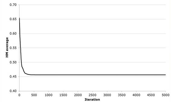
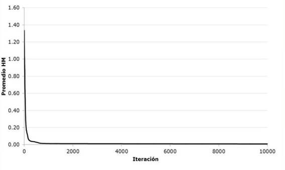
Throughout the total number of iterations the value of the optimization function represented by equation 17 shown in Figure 4 was recorded; in the same way, the optimization function evaluated in the 40 harmonies of the harmonic memory was averaged as shown in Figure 5.

Gumbel Mixed
Next, the same algorithm is used to carry out the optimization process of the Gumbel Mixed probability distribution or of two populations. The algorithm performs the most unfavorable harmonic modification contained in the harmonic memory and stochastically modifies one of the decision variables. That is, it modifies the four parameters of scale and location as well as the association parameter P. The algorithm carries out the exploration of the solution space as shown in Figures 6 and 7, defining a horizontal trend by the successive repetition of the optimal value of the parameter in the evaluated harmony, while the isolated values represent the stochastic values generated in the convergence process. Table 6 shows the adjusted values of the five parameters that result from this procedure, as well as the adjustment error. Comparing adjustments moments, Rosenbrock and Harmonica search for historical data of Santa Cruz hydrometric station shown in Figure 8.


Table 6 Parameters for the Gumbel Mixed function fit for the recording of annual maximum flows of the Santa Cruz hydrometric station, Sinaloa. Mexico.
| Methodology | P | λ1 (m3/s) | ε1 (m3/s) | λ2 (m3/s) | ε2 (m3/s) | EE |
|---|---|---|---|---|---|---|
| Moments | 0.784 | 863.652 | 200.780 | 3,133.625 | 1,369.655 | 542.022 |
| Rosenbrock | 0.850 | 769.051 | 296.580 | 3,037.430 | 1,022.059 | 407.024 |
| B. Harmonic | 0.824 | 788.796 | 281.276 | 2,850.544 | 1,436.975 | 400.008 |

Figure 8 Gumbel Mixed function fit for data from the Santa Cruz,
Sinaloa station. Method of moments (  ),
Rosenbrock's algorithm ( ) and
Harmonic Search ( ).
),
Rosenbrock's algorithm ( ) and
Harmonic Search ( ).
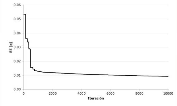
Figures 9 and 10 show the evolution of the value of the optimization function represented by equation 17 for the case of the Gumbel Mixed univariate distribution. The evolution in the solution space of the aleatory search of the harmonics carried out by the proposed algorithm is presented in a sequence in Figures 11 to 15.


Gómez et al., (2010) present a classic example of the numerical adjustment of a Gumbel Mixed distribution. In order to exemplify the proposed procedure, the historical data of station 12504 called La Cuña in the state of Jalisco are used. The parameters of the algorithm were xU=[1, 3000, 3000, 3000, 3000], xL=[1,0,0,0,0], HMS=30, NI=10000, HMCR=0.90, PAR=0.38; B=(xU-xL)/NI to start the pseudo-code of Table 2.
Table 7 shows the value of the five adjustment parameters for the Gumbel Mixed function for the record of annual maximum flows of the La Cuña hydrometric station, Jalisco. Figure 16 shows the accuracy in adjusting the extreme values when the harmonic estimation search parameters Gumbel Mixed univariate distribution is used. In the same way as for the data of the Santa Cruz station, Figures 17 and 18 show the evolution in the convergence of the optimization function.
Table 7 Parameters for the Gumbel Mixed function fit for the recording of maximum annual flows of the La Cuña hydrometric station, Jalisco Mexico.
| Methodology | P | λ1 (m 3 /s) | ε1 (m 3 /s) | λ2 (m 3 /s) | ε2 (m 3 /s) | EE |
|---|---|---|---|---|---|---|
| Gomez et al. 2010 | 0.8965 | 292.311 | 157.143 | 1271.095 | 424.786 | 80.200 |
| Harmonic Search | 0.8674 | 296.599 | 170.766 | 713.726 | 782.383 | 66.082 |

Figure 16 Optimization of the Mixed Gumbel function for the Cuña, Jalisco station using the Harmonic Search algorithm.
On the other hand, Figures 19 to 23 show the aleatory behavior of the location and scale parameters for the cyclonic and non-cyclonic samples.


Discussion
The first case study referred to the Santa Cruz hydrometric station, in which the Gumbel distribution function of one population was first adjusted to contrast the Harmonic Search algorithm with the conventional methodologies of Moments and Maximum Likelihood. An important decrease in the value of the Standard Adjustment Error could be observed, although graphically a better performance of the adjustment by Moments and even by Maximum Likelihood is appreciated. However, it should be noted that there was a decrease in the magnitude of EE for the Harmonic Search algorithm. This better adjustment is mainly due to the fact that good performance is shown in the area of flows with a value of the reduced variable of less than 1.5. That is, it does not comply with the maximum historical flows of the series, generating an important forecast error in the final zone of the series.
Regarding the convergence of the algorithm, it is observed in Figure 4 that very few iterative processes are required to reach the optimal solution. Similarly in Figure 5 you can see the mean of the 40 harmonies or combinations of values of the evaluated variables where, when the worst harmony is eliminated, the remaining 39 begin to reduce the value of the optimization function when compared with each other. Which guarantees a fast convergence, although the stochastic exploration of the solution space defined by the threshold values in the decision variables and the number of iterations continues. In Figures 6 and 7 shows how during the search values corresponding to the best solution to the problem harmony or visually generating a trend line aligned.
As the optimization of the Gumbel Mixed function develops, we can again appreciate that it decreases the value of the Standard Adjustment Error with respect to the methods at the moment and the Rosenbrock Algorithm. Regarding the latter, the variation is minimal in the result but visually we can see that the adjustment improves its performance in the region of the maximum flows of the series but presents difficulties in the zone of the minimum flows. Likewise, it presents a good convergence performance requiring approximately 2000 iterations of the 10000 performed to optimize the five parameters of the objective function, (the evolution of the iterations can be seen in the Figures 9 and 10) since the difference of equation 17 quickly decreases when evaluating the harmonic harmonics of 40, whereby the parameters ε 1 , ε 1 and ε 2 show greater stability in the stochastic exploration process to define its value optimized unlike ε 2 and P, this last parameter being the one that requires more iterations to identify the minimum in correlation with the rest.
Finally, by increasing the size of the time series of maximum flows we can see in Figure 16 that the adjustment by means of the Harmonic Search algorithm improves significantly in the area of the smaller flows without neglecting the region of higher flows with which there is a reduced value of the Standard Adjustment Error. in this particular case we can observe greater stability in the determination of the parameters P , ε 1 and ε 1 , the last two associated with the non-cyclonic data, while the parameters ε 2 and ε 2 corresponding to cyclonic data show a greater imbalance, particularly in the first 2000 iterations gradually and gradually reducing.
Conclusions
The results show that the harmonic search algorithm can optimize the Gumbel distribution function of both one and two populations (Gumbel Mixed), in the first case without a notable difference compared to conventional methods of adjustment even without improving the trend ordered by the reduced variable. On the other hand, when considering non-cyclonic and cyclonic populations, a significant increase in the performance of the proposed algorithm is observed to optimize the adjustment and decrease the adjustment error; which is enhanced by the use of extensive historical data series, so that their area of opportunity is located precisely in large registers. The Harmonic Search must be considered a viable option and of generalized application for the future estimation of parameters of probability distributions used in hydrology.
Referencias
Ahn, K., & Merwade, V. (2016). The effect of land cover change on duration and severity of high and low flows. Hydrological Processes, 31(1), 133-149. doi: 10.1002/hyp.10981 [ Links ]
Ahn, K., & Palmer, R. (2016). Use of a nonstationary copula to predict future bivariate low flow frequency in the Connecticut River basin. Hydrological Processes, 30(19), 3518-3532. doi: 10.1002/hyp.10876 [ Links ]
Al Aamery, N., Fox, J., Snyder, M., & Chandramouli, C. (2018). Variance analysis of forecasted streamflow maxima in a wet temperate climate. Journal of Hydrology, 560, 364-381. doi: 10.1016/j.jhydrol.2018.03.038 [ Links ]
Amin, M., Rizwan, M., & Alazba, A. (2014). Comparison of mixed distribution with EV1 and GEV components for analyzing hydrologic data containing outlier. Environmental Earth Sciences, 73(3), 1369-1375. doi: 10.1007/s12665-014-3490-4 [ Links ]
Arnaud, P., Cantet, P., & Odry, J. (2017). Uncertainties of flood frequency estimation approaches based on continuous simulation using data resampling. Journal of Hydrology, 554, 360-369. doi: 10.1016/j.jhydrol.2017.09.011 [ Links ]
Ashkar, F., El-Jabi, N., & Sarraf, S. (1991). Study of hydrological phenomena by extreme value theory. Natural Hazards, 4(4), 373-388. doi: 10.1007/bf00126645 [ Links ]
Ayantobo, O., Li, Y., Song, S., Javed, T., & Yao, N. (2018). Probabilistic modelling of drought events in China via 2-dimensional joint copula. Journal of Hydrology, 559, 373-391. doi: 10.1016/j.jhydrol.2018.02.022 [ Links ]
Bardsley, W. (2016). Cautionary note on multicomponent flood distributions for annual maxima. Hydrological Processes, 30(20), 3730-3732. doi: 10.1002/hyp.10886 [ Links ]
Borga, M., Vezzani, C., & Fontana, G. (2005). Regional Rainfall Depth-Duration-Frequency Equations for an Alpine Region. Natural Hazards, 36(1-2), 221-235. doi: 10.1007/s11069-004-4550-y [ Links ]
Campos-Aranda, D. F. (2003). Introducción a los Métodos Numéricos: Software en Basic y aplicaciones en hidrología superficial. Capítulo 5: Ajuste de curvas, pp. 93-127 y Capitulo 9. Optimización numérica, pp. 172-211, San Luis Potosí, Librería Universitaria Potosina. [ Links ]
Campos-Aranda, F. (1989). Estimación de los parámetros óptimos de la distribución Gumbel mixta por medio del algoritmo de Rosenbrock. Ingeniería Hidráulica en México, vol. Ene-Abr, pp. 9-18 [ Links ]
Campos-Aranda, F. (1994). Aplicación del Método del Índice de Crecientes en la Región Hidrológica Número 10, Sinaloa. Ingeniería Hidráulica en México , vol. IX, núm. 3, pp. 41-55 [ Links ]
Chen, L., & Singh, V. (2018). Entropy-based derivation of generalized distributions for hydrometeorological frequency analysis. Journal of Hydrology, 557, 699-712. doi: 10.1016/j.jhydrol.2017.12.066 [ Links ]
Chow, V. T. (1964). Statistical and probability analysis of hydrologic data. Section 8, part I frequency analysis. In: Handbook of applied hydrology. McGraw-Hill, Nueva York. [ Links ]
Cuevas, E., Ortega-Sánchez, N. (2013). El algoritmo de búsqueda armónica y sus usos en el procesamiento digital de imágenes. Computación y sistemas vol. 17 No. 4, pp. 543-560. Doi: 10.13053/CyS-17-4-2013-007 [ Links ]
Díaz-Delgado C., Bâ K., y Trujillo-Flores E. (1999). Las funciones Beta-Jacobi y Gamma-Laguerre como métodos de análisis de valores hidrológicos extremos. Caso de precipitaciones máximas anuales. Ingeniería Hidráulica en México, vol. XIV, núm. 2, pp. 39-48 [ Links ]
Escalante-Sandoval, C. (2007). Application of bivariate extreme value distribution to flood frequency analysis: a case study of Northwestern Mexico. Natural Hazards, 42(1), 37-46. doi: 10.1007/s11069-006-9044-7 [ Links ]
Escalante-Sandoval, C. (2013). Estimation of Extreme Wind Speeds by Using Mixed Distributions. Ingeniería Investigación y Tecnología, XIV(2), 153-162 [ Links ]
Escalante-Sandoval, C., y Domínguez-Esquivel, J. (2001). Análisis regional de precipitación con base en una distribución bivariada ajustada por máxima entropía. Ingeniería Hidráulica en México, vol. XVI, núm. 3, pp. 91-102 [ Links ]
Fogel, L., Owens, A., & Walsh, M. (1966). Artificial intelligence through simulated evolution. Chichester, WS, UK: Wiley. [ Links ]
Geem, Z. W., Kim, J. H., & Loganathan, G. V. (2001). A new heuristic optimization algorithm: Harmony search. Simulation, 76(2), 60-68. doi: 10.1177/003754970107600201 [ Links ]
Glover, F. (1977). Heuristics for integer programming using surrogate constraints. Decision Sciences, 8(1), 156-166. doi: 10.1111/j.1540-5915.1977.tb01074.x [ Links ]
Gómez, J., Aparicio, J., y Patiño, C. (2010). Manual de análisis de frecuencias en hidrología. Instituto Mexicano de Tecnología del Agua. Jiutepec, Morelos. [ Links ]
Grünthal, G., Thieken, A., Schwarz, J., Radtke, K., Smolka, A., & Merz, B. (2006). Comparative Risk Assessments for the City of Cologne - Storms, Floods, Earthquakes. Natural Hazards, 38(1-2), 21-44. doi: 10.1007/s11069-005-8598-0 [ Links ]
Gumbel, E. J. (1960). Distributions del valeurs extremes en plusieurs dimensions, Publications de L‘Institute de Statistique, Paris, Vol. 9, 171-173. [ Links ]
Gutiérrez-López, A., & Ramírez, A. (2005). Predicción hidrológica mediante el Método de la Avenida Índice para dos poblaciones. Ingeniería Hidráulica en México, vol. XX, núm. 2, pp. 37-47 [ Links ]
Holland, J. H. (1975) Adaptation in Natural and Artificial Systems. University of Michigan Press, Ann Arborr. (2nd Edition, MIT Press, 1992.) [ Links ]
Huang, J., Li, Y., Yin, J., & Mcbean, E. (2016). Precipitation regional extreme mapping as a tool for ungauged areas and the assessment of climate changes. Hydrological Processes, 30(12), 1940-1954. doi: 10.1002/hyp.10743 [ Links ]
Jenkinson, A. F. (1969). Estimation of maximum floods (Technical Note No. 98, ch. 5). Geneva, Switzerland: World Meteorological Organization. [ Links ]
Joshi, S., Jayadeva, Ramakrishnan, G., & Chandra, S. (2012). Using Sequential Unconstrained Minimization Techniques to simplify SVM solvers. Neurocomputing, 77(1), 253-260. doi: 10.1016/j.neucom.2011.07.010 [ Links ]
Karim, F., Petheram, C., Marvanek, S., Ticehurst, C., Wallace, J., & Hasan, M. (2015). Impact of climate change on floodplain inundation and hydrological connectivity between wetlands and rivers in a tropical river catchment. Hydrological Processes, 30(10), 1574-1593. doi: 10.1002/hyp.10714 [ Links ]
Kirkpatrick, S., Gelatt, C., & Vecchi, M. (1983). Optimization by Simulated Annealing. Science, 220(4598), 671-680. doi: 10.1126/science.220.4598.671 [ Links ]
Koutsoyiannis, D. (2004). On the appropriateness of the Gumbel distribution for modelling extreme rainfall (solicited). Hydrological Risk: recent advances in peak river flow modelling, prediction and real-time forecasting. Assessment of the impacts of land-use and climate changes. Edited by Brath, A., Montanari, A., and Toth, E. Bologna, 303-319, doi:10.13140/RG.2.1.3811.6080, Editoriale Bios, Castrolibero, Italy. [ Links ]
Kuester, J., & Mize, J. (1973). Optimization Techniques with Fortran, ROSENB algorithm, New York, McGraw-Hill Book Co. pp:320-330 [ Links ]
Lee, K., & Geem, Z. (2005). A new meta-heuristic algorithm for continuous engineering optimization: harmony search theory and practice. Computer Methods in Applied Mechanics and Engineering, 194(36-38), 3902-3933. doi: 10.1016/j.cma.2004.09.007 [ Links ]
Lilienthal, J., Fried, R., & Schumann, A. (2018). Homogeneity testing for skewed and cross-correlated data in regional flood frequency analysis. Journal of Hydrology, 556, 557-571. doi: 10.1016/j.jhydrol.2017.10.056 [ Links ]
Mélèse, V., Blanchet, J., & Molinié, G. (2018). Uncertainty estimation of Intensity-Duration-Frequency relationships: A regional analysis. Journal of Hydrology, 558, 579-591. doi: 10.1016/j.jhydrol.2017.07.054 [ Links ]
Montaseri, M., Amirataee, B., & Rezaie, H. (2018). New approach in bivariate drought duration and severity analysis. Journal of Hydrology, 559, 166-181. doi: 10.1016/j.jhydrol.2018.02.018 [ Links ]
Öztürk, S., Bayrak, Y., Çınar, H., Koravos, G., & Tsapanos, T. (2008). A quantitative appraisal of earthquake hazard parameters computed from Gumbel I method for different regions in and around Turkey. Natural Hazards, 47(3), 471-495. doi: 10.1007/s11069-008-9234-6 [ Links ]
Phillips, R., Samadi, S., & Meadows, M. (2018). How extreme was the October 2015 flood in the Carolinas? An assessment of flood frequency analysis and distribution tails. Journal of Hydrology, 562, 648-663. doi: 10.1016/j.jhydrol.2018.05.035 [ Links ]
Qi, W., & Liu, J. (2018). A non-stationary cost-benefit based bivariate extreme flood estimation approach. Journal of Hydrology, 557, 589-599. doi: 10.1016/j.jhydrol.2017.12.045 [ Links ]
Qian, L., Wang, H., Dang, S., Wang, C., Jiao, Z., & Zhao, Y. (2017). Modelling bivariate extreme precipitation distribution for data-scarce regions using Gumbel-Hougaard copula with maximum entropy estimation. Hydrological Processes, 32(2), 212-227. doi: 10.1002/hyp.11406 [ Links ]
Raynal-Villaseñor, J. (1997). Sobre el uso del dominio de atracción para la identificación de distribuciones de valores extremos para máximos. Ingeniería Hidráulica en México, vol. XII, núm. 2, pp. 57-62 [ Links ]
Rosenbrock, H. H. (1960). An automatic method for finding the greatest or least value of a function. The Computer Journal, 3:175-184. doi:10.1093/comjnl/3.3.175 [ Links ]
Rossi, F., Florentino, M., & Versace, P. (1984). Two-Component Extreme Value Distribution for Flood Frequency Analysis. Water Resources Research 20(7). 847-856. doi:10.1029/WR020i007p00847. [ Links ]
Schulz, K., & Bernhardt, M. (2016). The end of trend estimation for extreme floods under climate change?. Hydrological Processes, 30(11), 1804-1808. doi: 10.1002/hyp.10816 [ Links ]
Smitha, P., Narasimhan, B., Sudheer, K., & Annamalai, H. (2018). An improved bias correction method of daily rainfall data using a sliding window technique for climate change impact assessment. Journal of Hydrology, 556, 100-118. doi: 10.1016/j.jhydrol.2017.11.010 [ Links ]
So, B., Kim, J., Kwon, H., & Lima, C. (2017). Stochastic extreme downscaling model for an assessment of changes in rainfall intensity-duration-frequency curves over South Korea using multiple regional climate models. Journal of Hydrology, 553, 321-337. doi: 10.1016/j.jhydrol.2017.07.061 [ Links ]
Strupczewski, W., Kochanek, K., & Bogdanowicz, E. (2017). Historical floods in flood frequency analysis: Is this game worth the candle?. Journal of Hydrology, 554, 800-816. doi: 10.1016/j.jhydrol.2017.09.034 [ Links ]
Tao, S., Dong, S., Wang, N., & Guedes-Soares, C. (2013). Estimating storm surge intensity with Poisson bivariate maximum entropy distributions based on copulas. Natural Hazards, 68(2), 791-807. doi: 10.1007/s11069-013-0654-6 [ Links ]
Tosunoglu, F., & Can, I. (2016). Application of copulas for regional bivariate frequency analysis of meteorological droughts in Turkey. Natural Hazards, 82(3), 1457-1477. doi: 10.1007/s11069-016-2253-9 [ Links ]
Van de Vyver, H. (2018). A multiscaling-based intensity-duration-frequency model for extreme precipitation. Hydrological Processes. doi: 10.1002/hyp.11516 [ Links ]
Vu, M., Raghavan, V., & Liong, S. (2016). Deriving short-duration rainfall IDF curves from a regional climate model. Natural Hazards, 85(3), 1877-1891. doi: 10.1007/s11069-016-2670-9 [ Links ]
Yan, L., Xiong, L., Liu, D., Hu, T., & Xu, C. (2016). Frequency analysis of nonstationary annual maximum flood series using the time-varying two-component mixture distributions. Hydrological Processes, 31(1), 69-89. doi: 10.1002/hyp.10965 [ Links ]
Yang, J., Chang, J., Wang, Y., Li, Y., Hu, H., & Chen, Y. (2018). Comprehensive drought characteristics analysis based on a nonlinear multivariate drought index. Journal of Hydrology, 557, 651-667. doi: 10.1016/j.jhydrol.2017.12.055 [ Links ]
Yue, S. (2000). The Gumbel Mixed Model Applied to Storm Frequency Analysis. Water Resources Management, 14(5), 377-389. doi: 10.1023/a:1011124423923 [ Links ]
Zhang, R., Chen, X., Wang, H., Cheng, Q., Zhang, Z., & Shi, P. (2017). Temporal change of spatial heterogeneity and its effect on regional trend of annual precipitation heterogeneity indices. Hydrological Processes, 31(18), 3178-3190. DOI: 10.1002/hyp.11225 [ Links ]
Received: August 03, 2018; Accepted: August 08, 2018
 Este es un artículo publicado en acceso abierto bajo una licencia
Creative Commons
Este es un artículo publicado en acceso abierto bajo una licencia
Creative Commons
