


Serviços Personalizados
Journal
Artigo
 texto em
  Inglês (pdf)
 Artigo em XML
 Referências do artigo
 Enviar este artigo por email
Indicadores
-
 Citado por SciELO
 -
 Acessos
Links relacionados
-
 Similares em
SciELO
Similares em
SciELO
Compartilhar

 Permalink
Tecnología y ciencias del agua
versão On-line ISSN 2007-2422
Tecnol. cienc. agua vol.9 no.4 Jiutepec Jul./Ago. 2018 Epub 24-Nov-2020
https://doi.org/10.24850/j-tyca-2018-04-06
Articles
Hydrological assessment of the Teapa River basin, using the MIKE SHE model
1Colegio de Postgraduados, Postgrado en Hidrociencias, Montecillo, Estado de México, México, atm.marco@gmail.com
2Colegio de Postgraduados, Programa de Hidrociencias, Montecillo, Estado de México, México, nikolski@colpos.mx
3Manejo Integral de Cuencas S.A. de C.V., Texcoco, México, maeugenia0401@hotmail.com
4Colegio de Postgraduados, Programa de Hidrociencias, Montecillo, Estado de México, México, mmario@colpos.mx
The MIKE SHE hydrological model was applied by the present work in order to simulate water runoff from the Teapa River basin in southeastern Mexico. The basin has a humid tropical climate, high slopes, and is relatively little altered by human activities. There is relatively detailed information on climatic conditions, topography, vegetation, and soils in the basin, as well as data on the hydrologic regime of Teapa River. The MIKE SHE model is preferible because of its high capacity to process detailed characteristics of the river basin. The process to simulate the Teapa River’s hydrological regime involved two calculation stages. First, calibration of the model by means of some of its parameters, initially determined and related with hydrophysical properties of soils and hydraulic roughness of the surface, for a better fit between calculated and observed river discharges. Then, validation of the model by comparing calculated and observed river discharges. The results of the simulation showed that the MIKE SHE model validation process resulted in a rather good fit between the calculated and observed mean and maximum monthly discharges from the Teapa River, with a determination coefficient of R 2 = 0.81. However, the calculated and observed daily discharges did not result in a good fit, with R 2 = 0.62. A large number of model parameters, each of which presumably had an error, can possibly explain such a relatively low fit for the daily discharges.
Keywords Hydrologic modelling; distributed models; MIKE SHE
En el presente trabajo se ha aplicado el modelo hidrológico MIKE-SHE, para simular procesos de escorrentía de agua de la cuenca hidrológica del río Teapa, en el sureste de México. La cuenca tiene un clima tropical húmedo, altas pendientes y una escasa presencia de núcleos urbanos. Existe información detallada sobre las condiciones climáticas, topografía, de vegetación y suelos de la cuenca, así como datos del régimen hidrológico del río Teapa. Se ha implementado el modelo MIKE-SHE, principalmente por la gran capacidad de procesamiento de la información detallada de las cuencas. El proceso de simulación del régimen hidrológico del río Teapa comprende dos etapas de cálculo: la calibración del modelo, que tiene como finalidad obtener un buen ajuste entre los datos observados y los calculados, lo cual se logra mediante modificación de algunos de los parámetros iniciales relacionados con las propiedades físicas de los suelos y con la rugosidad hidráulica de la superficie y cauces; la validación del modelo consiste en la aplicación del mismo en un periodo sin calibración y la comparación de los gastos calculados y observados. Los resultados de la simulación señalan que en el proceso de validación del modelo MIKE-SHE se logró un ajuste entre los gastos del río Teapa medios y máximos mensuales, obteniendo un coeficiente de determinación R 2 = 0.81. Sin embargo, no se ha logrado buen ajuste de los gastos diarios con R 2 = 0.62.
Palabras clave modelación hidrológica; modelos distribuidos; MIKE-SHE; escurrimiento superficial
Introduction
The hydrological Teapa River basin, in southeastern Mexico, presents problems with flooding related to the fast growth of the flows in streams and rivers after torrential rains with high intensities, banks with high slopes, and alterations in the primary vegetation.
To prevent floods and mitigate their effects, it is necessary to estimate the probability and magnitude of the maximum flows in the rivers. Such estimates can be made using a statistical analysis of the observations data of the flows, or in case of a lack of data, using a mathematical simulation of the flow formation process in channels.
There are different simulation models for these processes, which are based on different principles. The most important is the level of reliability of the flows or water levels calculated. In order to verify the level of reliability of the calculated hydrological regime of a channel, the hydrometric stations need to have observation data continuously and for a sufficiently long period (years). It is also necessary to have objective and representative information about the conditions that influence and determine water runoff in a hydrological basin, such as: topography, climate, soils, vegetation, land use, and the hydrographic network. The Teapa River basin has the information needed to simulate the process of water runoff using distributed models and on a physical basis. In addition, there is very little urban area in this basin, which simplifies the simulation process.
The MIKE SHE model has a large capacity for processing the specific characteristics of the basin, such as meteorological, topographical, and hydrological conditions (DHI, 2007). Given this processing capacity, the objective of this work was to calibrate and validate the MIKE SHE hydrological model in the Teapa River basin in southeastern of Mexico.
Material and methods
Study area description
The Teapa River basin begins in the northern mountains of Chiapas state, in the municipality of Rayon. For the case of this study, the site of the Teapa hydrometric station (30032) was used as the outlet point of the basin. The extreme coordinates of the basin are 17 ° 34'5.24 " and 17 ° 10'58.03" north latitude and 92 ° 54'19.9" and 93 ° 64'54.83" west longitude. The Teapa River basin has a total drainage area of 430.7 km2. The order of classification of the Teapa River flows indicates that the main channel corresponds to the VI order, the Río Negro River tributary corresponds to the V order, San José River, La Sierra River, Moquimba River, and Jucubia River correspond to the IV order (INEGI, 2010). The main channel has an average slope of 22% and an elevation difference of 2 320 m.
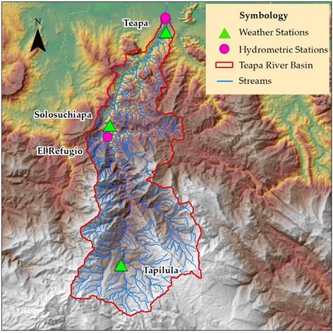
The predominant climate condition in the Teapa River basin corresponds to a warm humid climate with rains in summer and part of autumn. These rains are strongly influenced by the presence of tropical cyclones. It is also possible to identify a dry season because of the rainfall distribution in the Sierra Madre of Chiapas. The main climatic differences in the area correspond to an increase in winter rains, produced mainly by the influence of the "Nortes" that produce orographic rains on the slopes and part of the plains (García, 1988).
The land use and vegetation in the Teapa River basin are mostly cultivated pastures that, with an area of 207 km2, represent 48% of the the territory. The second largest land use in terms of area is rainfed agriculture, which represents 18%, with 81 km2. The rest of the basin's surface is divided into different types of land use and vegetation, mostly secondary vegetation associated with tropical rainforests and tropical montane cloud forests (INEGI, 2014a).
Luvisols are the predominant group of soils in the Teapa River basin. The main characteristic of these soils is a higher clay content in the subsoil than in the topsoil, as a result of rainy weather. Giventhe physiographic variability of the area, different subgroups of luvisols can be found. However, the endoleptic luvisols are more common due to the presence of lithic phases in the region. Most of the area in the basin that contains luvisols supports cultivated pastures, and rainfed agriculture can be cultivated ona smaller proportion (INEGI, 2014b).
Hydrologic models description
There are many different ways of classifying hydrological models. The basic classification separates the models into lumped models and distributed models, and a second classification separates the models into stochastic models and deterministic models (Beven, 2001). The MIKES SHE model is a distributed and stochastic model.
The lumped models consider the basin as a unit, where each of the variables represents the average values of the catchment area. Distributed models produce calculations by dividing the surface into a grid composed of a large number of individual cells. Each cell can contain different values of the evaluated characteristics, and the equations of the model are associated with each cell.
In general, deterministic models permit only one outcome from a simulation, with one set of inputs and parameter values. On the other hand, stochastic models allow for some randomness in the possible outcomes due to uncertainty in the input variables. The main objective of the stochastic models is to be able to predict future events with certain accuracy, based on sequential patterns in the flow of the streams (Klemes, 1982; Klemes, 1988).
An important consideration when using stochastic models is that they assume the seasonality of rain and runoff, which means that future rainfall and runoff series will have the same statistical distribution as in the past.
The main characteristics of the distributed models are:
The variable and heterogeneous character of the catchment is conserved as a result of the number of hydrological response units with homogeneous characteristics.
The hydrological response of the basin is the result of the integration of the hydrological response of the individual units.
Each unit is assigned variables and parameters that describe the typical climate, topography, soils, and vegetation for that unit.
It is possible to obtain hydrological simulations with high correlations because linear relationships are not included in the process.
The main disadvantages of distributed models are:
They are more complex than lumped models; however, more complex models are not necessarily better than simple models.
The division of a basin into theoretically homogeneous units is complicated due to the physical characteristics of each unit, their interactions for differently sized units vary, and information cannot necessarily be scaled.
MIKE SHE model description
The European Hydrological System (SHE) is a general system of modeling that is completely distributed and physically based. It can independently simulate the entire hydrological cycle or any of its terrestrial phases (Abbott, Bathurst, Cunge, O´Connell, & Rasmussen, 1986a).
The European hydrological system was initially developed in 1977by three European organizations: the Danish Hydraulic Institute (DHI), the British Institute of Hydrology, and SOGREAH, a French consulting company.
The European Hydrological System is the integration of a series of models, considering as the most important the MIKE SHE model and the MIKE 11 model, which together make it possible to characterize the behavior of river basins (DHI, 2004).
The MIKE SHE is physically based in the sense that the hydrological processes of water movement are modelled by mass and energy conservation equations, or by empirical equations derived from independent experimental research. The spatial distribution of the model is obtained from the horizontal representation of the area, according to an orthogonal grid network, and vertically, by a column of information layers in each grid square (Abbott, Bathurst, Cunge, O’Connel, & Rasmussen, 1986b).
The physical basis of the model makes it possible to include the topography, vegetation, soil, and climate characteristics. The distributed nature of the model permits spatial and temporal variations in each of the parameters in the set of information, such as soil profiles, land use, drainage practices, evapotranspiration, and surface runoff (Abbott et al., 1982).
With the aim of adapting to the different modeling needs of users, the SHE system is able to adapt to the type of hydrological problem and its scope, so the level of complexity of the modeling is variable. This is achieved with a modular structure of the model (DHI, 2004). Rhese modules are:
Snowmelt module
Canopy interception module
Evapotranspiration module
Overland flow module
Channel flow module
Saturated and unsaturated flow module
Each hydrological process is linked to a component of the model, so it is possible to simulate the entire hydrological cycle, or only the portion of interest.
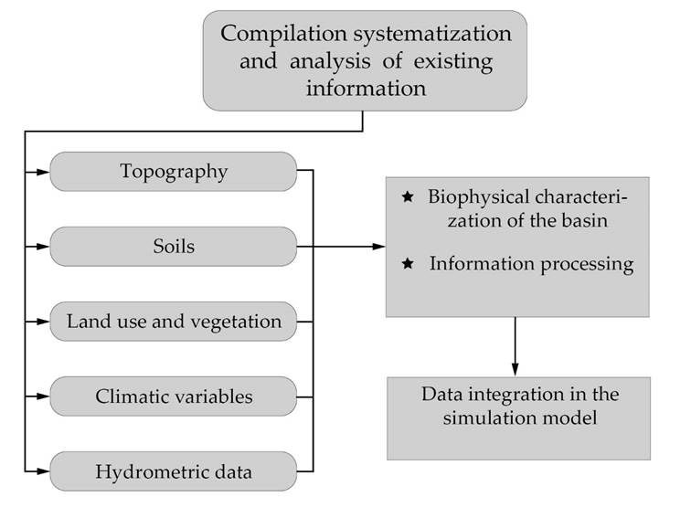
Integration of information in the MIKE SHE / MIKE 11 model
The MIKE SHE model is based on the physical laws of nature as well as on each of the representative data of the basin. The information used in the development of this work is represented with a general scheme for the purpose of processing the information and its integration in the model.
The topographic information used to perform the present work has two main sources:the digital terrain model LIDAR and the Continuum of Mexican Elevations CEM 3. Both are generated by the INEGI (INEGI, 2010).
To determine the runoff area of the basin, the Mexican elevation continuum CEM 3 by INEGI was used, with which the location of the basin’s boundary was obtained. It considered the location of the conventional hydrometric station “Río Teapa,” with identification number 30032, as the outlet point (INEGI, 2013).
The determination of the natural channels of the Teapa river basin was made by processing the LIDAR digital terrain model with a resolution of five meters per pixel, and considering a minimum contribution area of 20 hectares for the first-order channels. A total of 51 channels with an accumulated length of 725.3 Km were obtained.
The processing of the cross sections was made based on the point mesh of the LIDAR digital terrain model, adjusting the elevations from the datum obtained from the CEM3 elevation model. A distance between sections of 200 m was used, including an opening section and a closing at the confluences of the different natural channels. In total, 1 161 cross-sections in the hydrographic network were processed.
In order to standardize the available information related to the existing soil units in the Teapa River basin, the hydrological characteristics of the soils in the model were integrated using two main sources of information: 1) soil maps with a scale of 1:50 000, from INEGI; and 2) the series I and II from the soil profile databases (INEGI, 1988; INEGI, 2004a; INEGI, 2004b; INEGI, 2014a). The soil group and subgroup polygons were used as a general structure. For the input of the information in the model, the resulting polygons were related to the reported physical and chemical characteristics of the soil profiles.
The hydrologic characteristics of moisture content at saturation, moisture content at field capacity, moisture content at the point of permanent wilting, and hydraulic conductivity were calculated using the method to estimate soil hydraulic properties for hydrological solutions (Saxton, & Rawsl, 2006), with organic matter, textural fractions, and compaction degree values.
The identification of the vegetation types in the Teapa River basin was made by visual classification of the LANDSAT satellite image for the periods studied, and making a comparison with the types of vegetation reported by INEGI in the series IV and V of the land use and vegetation map.
The integration of the different climate variables in the MIKE SHE model was done with the introduction of different time series, whichwere processed individually from the information available from the conventional weather stations and the automated weather station in the basin.
The eventual precipitation data was analyzed, which was obtained from the automated weather station, with a measurement interval of 10 minutes. A total of 752 rainfall events were identified during the period between January 2011 to March 2014. The mass curve obtained from this analysis makes it possible to evaluate and adjust the daily precipitation records reported by the conventional weather stations, obtaining an adequate time series for use in the simulation process with the MIKE SHE model.
The daily evapotranspiration time series were obtained from the Hargreaves equation (Hargreaves & Samani, 1985), which evaluates the potential evapotranspiration from extreme temperatures and solar radiation data.
The integration of the hydrometric information in the model allows its calibration and validation, serving as a comparison between the results obtained from the model and the values measured in the field for the same period of time. In the Teapa River basin, two sites can be used to measure the hydrometric series in the basin. One site corresponds to the conventional hydrometric station, which constitutes the outlet point of the basin. The other is the automated hydrometric station, which serves as a comparative site for the hydrological evaluation.
The daily flow, the average monthly flow, and the maximum monthly flow recorded by the conventional hydrometric station serve as the main comparison values for the calibration and validation of the model. The instantaneous values of scale and speed reported by the automated hydrometric station make it possible to estimate the flow in the section where they are located, These flow values are considered comparative values because they do not represent a direct measurement of the flow in the channel and require a calibration process.
The records of the water elevation in the hydraulic section is a obtained from the OTT RLS elevation sensor located in the automated hydrometric station. This information has a measurement interval of 10 minutes, and the evaluation period was 08/06/2011 23:20 to 02/06/2013 16:40. The time series of surface velocity of the flow in the hydrometric section was obtained from the Kalesto speed sensor, for the same evaluation period.
Results and discussion
The results of a model can be used for different activities, such as making decisions about the management of water resourcesk or for research tasks. The models need to be scientifically strong, robust, and defensible (EPA, 2002).
The process for analyzing the results needs to be determined before beginning the development of the model, since it is necessary to clearly define the ASCE evaluation criteria (ASCE, 1993). In general, the statistical criteria have been widely used, some and specific statistics have been developed, as well as performance indices for the evaluation of the models (Donigian, Imhoff, & Bicknell, 1983). The evaluation of the The MIKE SHE model was evaluated in the present work based on Moriasi, Arnold, Van Liew, Bingner, Harmel and Vieth (Moriasi et al., 2007).
The hydrological evaluation of the Teapa River basin using the MIKE SHE model was made in two stages: calibration and validation of the model.
Model calibration
The period selected for the calibration of the model was from 1998 to 2000. The average daily flows, average monthly flows, and maximum monthly flows reported by the Teapa River hydrometric station 30032 were compared with the simulated flows.
The adjustment parameters of the calibration correspond to two components of the model: saturation hydraulic conductivity of the soil, saturation moisture (or porosity), field capacity moisture, wilting point moisture, and hydraulic surface roughness of the basin, which are responsible for the unsaturated flow zone and the surface flow component, respectively.
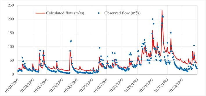
As can be observed, there is usually some adjusting of the dynamics of change over time of the daily calculated and observed flows. It is also observed that, periodically during the periods of moderate or weak flows, the calculated values of daily flows exceed the observed flows. It is also observed that during the periods of maximum flows the fit between the calculated and observed descharges is generally better.
The evaluation of the adjustment of the calculated daily flows compared to the observed daily flows in the period of calibration was carried out by analyzing the following statistical indicators: mean absolute error (MAE), root mean square error (RMSE), standard deviation residuals (STDres), determination coefficient R 2, and R 2 Nash Sutcliffe determination coefficient (Table 1).
Table 1 Results of the statistical estimation of the calibration quality of the MIKE SHE model in the process of calculating the daily flows of the Teapa River, Tabasco
| Time lapse | MAE | RMSE | STDres | R 2 | R 2 Nash Sutcliffe |
|---|---|---|---|---|---|
| 01/01/1998 a 31/12/2000 | 15.987 | 30.043 | 29.8588 | 0.72568 | 0.51662 |
| 01/01/1998 a 31/12/1998 | 11.049 | 22.539 | 22.5294 | 0.69343 | 0.46111 |
| 01/01/1999 a 31/12/1999 | 13.703 | 26.823 | 26.8137 | 0.81253 | 0.63732 |
| 01/01/2000 a 31/12/2000 | 24.648 | 39.962 | 38.3707 | 0.67158 | 0.40144 |
Note: MAE = mean absolute error; RMSE = root mean square error; STDres = Standard deviation residuals; R 2 = determination coefficient; R 2 Nash Sutcliffe = Nash Sutcliffe determination coefficient.
Through the results obtained, an evaluation was made of the average monthly flows and the maximum monthly flows, obtaining the following results.
The determination coefficient, R 2, between the average monthly flow discharge (calculated and observed) in the Teapa hydrometric station during the calibration period from 1998 to 2000 was equal to 0.84, which means a good fit between the calculated and observed values.
The determination coefficient between maximum monthly flows was 0.77, which means that there was a good fit between the calculated and observed maximum monthly flow in the calibration stage of the MIKE SHE model.
Model validation
The period selected for the calibration of the model was from 2003 to 2005. Daily flows, average monthly flows, and maximum monthly flows reported by the Teapa River hydrometric station 30032 were compared with the simulated flows.
The fit of the calculated daily flows compared with the observed daily flows in the validation period was evaluated in the same way as the calibration period, with the criteria MAE, RMSE, STDres, R 2 and Nash Sutcliffe R 2 (Table 2 and Figure 4).
Table 2 Results of the statistical estimation of the validation quality of the MIKE SHE model in the process of calculating the daily flows of the Teapa River, Tabasco.
| Time lapse | MAE | RMSE | STDres | R 2 | R 2 Nash Sutcliffe |
|---|---|---|---|---|---|
| 01/01/2003 a 31/12/2005 | 14.589 | 27.805 | 27.6196 | 0.66440 | 0.42777 |
| 01/01/2003 a 31/12/2003 | 20.032 | 32.613 | 31.8116 | 0.69775 | 0.43874 |
| 01/01/2004 a 31/12/2004 | 12.016 | 22.580 | 22.5796 | 0.67943 | 0.45729 |
| 01/01/2005 a 31/12/2005 | 11.772 | 27.396 | 27.2922 | 0.60199 | 0.35446 |
Note: MAE = mean absolute error; RMSE = root mean square error; STDres = Standard deviation residuals; R 2 = determination coefficient; R 2 Nash Sutcliffe = Nash Sutcliffe determination coefficient.
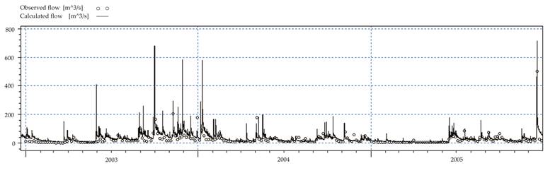
Figure 4 Comparison of the calculated daily flows and observed flows in the Teapa River hydrometric station during the 2003-2005 validation period.
As can be seen, there is a good correlation between the calculated flows and the observed flows, however the statistical values of the validation are lower than those obtained during the calibration process. As in the case of the calibration process, the average monthly and maximum flows in the validation period were evaluated, resulting in the following results (Figure 5).
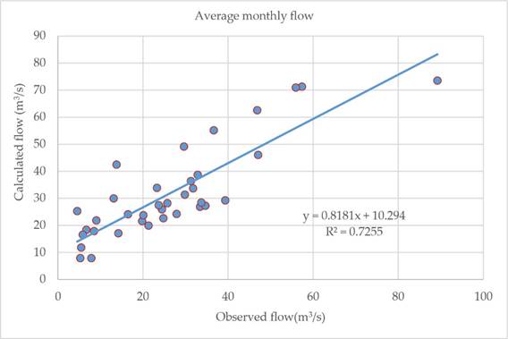
Figure 5 Correlation between calculated and observed average monthly flows for the Teapa hydrometric station during the validation period, from 2003 to 2005.
The determination coefficient, R 2, between the calculated and observed average monthly flow discharge in the Teapa hydrometric station during the validation period, from 2003 to 2005, was equal to 0.73, which was greater than daily flows ratio (0.63) and a little lower than the calibration period (0.84). In general, that means good fit between the calculated and observed values of the average monthly flows.
The maximum monthly and annual flows are of great importance since these flows are related to critical situations in natural streams: overflows, floods, and negative impacts. Considering this, a comparison was made of the calculated and observed maximum flows for the Teapa hydrometric station during the validation period, from 2003 to 2005.
A good fit was found between the calculated and observed dynamics of the maximum monthly flows time-series. For greater clarity, the correlation graph between the maximum calculated and observed flows at the Teapa hydrometric station during the validation period is presented.
The coefficient of determination for the maximum monthly flows was 0.81, which was higher than in the calibration period (0.77), and which means that there is a good fit between the calculated and observed maximum monthly flows in the calibration stage of the MIKE SHE model.
Conclusions
A good fit was found between the calculated and observed average and maximum monthly and annual discharge flows corresponding to the Teapa River, with a determination coefficient R 2 = 0.81 in the validation process of the MIKE SHE model. This means that this model can be used at least for conditions similar to the Teapa River basin, in order to estimate the risk of overflow and flooding due to high water levels. This can be used to support the planning, design, and evaluation of basin management scenarios, taking into account agricultural practices and possible modifications of the basin infrastructure that alter the hydrological conditions.
The rather low fit between the calculated and observed daily discharge flows during the validation process of the MIKE SHE model can be possibly explained by the large number of model parameters, each one of which can have some error.
The meteorological, hydrometric, and biophysical information in the area of influence of the Teapa River basin was sufficient to integrate, calibrate, and validate the physically-based hydrological MIKE SHE / MIKE 11 model.
Acknowledgements
We are thankful to the Organismo de Cuenca Frontera Sur (OCFS- CONAGUA) for access to the hydrometric and meteorological information used in our investigation.
REFERENCES
Abbott, M. B., Andersen, J. K., Havno, K., Jensen, K. H., Kroszynski, U. I., & Warren, I. R. (1982). Research and development for the unsaturated zone component of the European Hydrologic System-Systeme Hydrologique Europeen (SHE). En: Abbott M. B., & Cunge J. A. (eds.). Engineering Applications of Computational Hydraulics. London, UK: Pitman. [ Links ]
Abbott, M. B., Bathurst, J. C., Cunge, J. A., O’Connel, P.E., & Rasmussen, J. (1986a). An introduction to the European hydrological system - Systeme Hydrologique Europeen, "SHE", 1: History and philosophy of a physically-based, distributed modelling system. Journal of Hydrology, 87(1), 45-59. [ Links ]
Abbott, M. B., Bathurst J. C., Cunge J. A., O’Connel P.E., & Rasmussen J. (1986b). An introduction to the European hydrological system - Systeme Hydrologique Europeen, "SHE", 2: Structure of a physically-based, distributed modelling system. Journal of Hydrology, 87(1), 61-77. [ Links ]
ASCE, American Society of Civil Engineers. (1993). Criteria for evaluation of watershed models. Journal of Irrigation Drainage Engineering, 119(3), 429-442. [ Links ]
Beven, K. J. (2001). Rainfall-runoff modelling: The Primer (2nd ed.). London, UK: Wile-Blackwell. [ Links ]
DHI. (2004). MIKE SHE user manual. Horsholm, Denmark: Publ. Danish Hydraulic Institute. [ Links ]
DHI. (2007). MIKE SHE User Manual vol. 1: User Guide. DHI Water & Environment Publ. Recuperado de http://www.hydroasia.org/jahia/webdav/site/hydroasia/shared/Document_public/Project/Manuals/WRS/MIKE_SHE_UserGuide.pdf [ Links ]
Donigian, A. S., Imhoff, J. C., & Bicknell, B. R. (1983). Predicting water quality resulting from agricultural nonpoint-source pollution via simulation − HSPF. In: Agricultural Management and Water Quality. Ames, USA: Iowa State University Press. [ Links ]
EPA, United States Environmental Protection Agency. (2002). Guidance for quality assurance project plans for modeling. EPA QA/G-5M (Report EPA/240/R-02/007). Washington, DC, USA: United States Environmental Protection Agency, Office of Environmental Information. [ Links ]
García, E. (1988). Modificaciones al sistema de clasificación climática de Köppen (para adaptarlo a las condiciones de la República Mexicana). México, DF, México: Instituto de Geografía, Universidad Nacional Autónoma de México. [ Links ]
Hargreaves, G. H., & Samani, Z. A. (1985). Reference crop evapotranspiration from temperature. Applied Engineering in Agriculture, 1(2):96-99. Recuperado de http://dx.doi.org/10.13031/2013.26773. [ Links ]
INEGI, Instituto Nacional de Estadística y Geografía. (1988). Conjunto de las cartas de topografía, geología, uso de suelo y edafología, (escala 1:250 000 y 1:50 000) de la República Mexicana. Aguascalientes, México: Instituto Nacional de Estadística, Geografía e Informática. [ Links ]
INEGI, Instituto Nacional de Estadística y Geografía. (2004a). Conjunto de datos vectoriales de la serie topográfica y de recursos naturales escala. 1:1 000 000. Recuperado de http://www.inegi.org.mx/geo/contenidos/recnat/edafologia/PerfilesSuelo.aspx [ Links ]
INEGI, Instituto Nacional de Estadística y Geografía. (2004b). Conjunto de datos de perfiles de suelos escala Serie I y II Escala 1:250 000. Recuperado de http://www.inegi.org.mx/geo/contenidos/recnat/edafologia/ [ Links ]
INEGI, Instituto Nacional de Estadística y Geografía. (2010). Documento técnico descriptivo de la red hidrográfica escala 1:50 000. Edición: 2.0. Aguascalientes, México: Dirección General de Geografía y Medio Ambiente. [ Links ]
INEGI, Instituto Nacional de Estadística y Geografía. (2013). Continuo de Elevaciones Mexicano 3.0 (CEM 3.0). Recuperado de http://www.inegi.org.mx/geo/contenidos/datosrelieve/continental/continuoelevaciones.aspx [ Links ]
INEGI, Instituto Nacional de Estadística y Geografía. (2014a). Conjunto de datos vectoriales edafológicos. Escala 1:250 000, Serie II. Recuperado de http://www.inegi.org.mx/geo/contenidos/recnat/edafologia/vectorial_serieii.aspx [ Links ]
INEGI, Instituto Nacional de Estadística y Geografía. (2014b). Conjunto de datos vectoriales edafológicos, escala 1:250 000, Serie II. Recuperado de http://www.inegi.org.mx/geo/contenidos/recnat/edafologia/vectorial_serieii.aspx [ Links ]
Klemes, V. (1982). Empirical and causal models of hydrology. In: Scientific Basis of Water Resource Management (pp. 95-104). Washington, DC, USA: National Academy of Sciences. [ Links ]
Klemes, V. (1988). A hydrological perspective. Journal of hydrology, 100(1), 3-28. [ Links ]
Moriasi, D. N., Arnold, J. G., Van Liew, M. W., Bingner, R. L., Harmel, R. D., & Vieth, T. L. (2007). Model evaluation guidelines for systematic quantification accuracy in watershed simulations. Transactions of ASABE, 50(3), 885-900. [ Links ]
Saxton, K. E., & Rawls, W. (2006). Soil water characteristics estimates by texture and organic matter for hydrologic solutions. Soil Science Society of American Journal, 70, 1569-1578. [ Links ]
Received: July 08, 2016; Accepted: January 25, 2018
 Este es un artículo publicado en acceso abierto bajo una licencia
Creative Commons
Este es un artículo publicado en acceso abierto bajo una licencia
Creative Commons
