


Servicios Personalizados
Revista
Articulo
 texto en
  Inglés (pdf)
 Artículo en XML
 Referencias del artículo
 Enviar artículo por email
Indicadores
-
 Citado por SciELO
 -
 Accesos
Links relacionados
-
 Similares en
SciELO
Similares en
SciELO
Compartir

 Permalink
Tecnología y ciencias del agua
versión On-line ISSN 2007-2422
Tecnol. cienc. agua vol.9 no.2 Jiutepec mar./abr. 2018 Epub 24-Nov-2020
https://doi.org/10.24850/j-tyca-2018-02-06
Articles
Uncertainty in the outputs of a semi-distributed hydrological model
1Universidad Católica de la Santísima Concepción, Concepción, Chile, emunozo@ucsc.cl
2Universidad Católica de la Santísima Concepción, Concepción, Chile, jcgutierrez@ing.ucsc.cl
3Universidad Católica de la Santísima Concepción, Concepción, Chile, ptume@ucsc.cl
For proper water management, it is necessary to know both the flows simulated by a model and the uncertainty associated with them. This study seeks to quantify the uncertainty in the flows simulated by a hydrological model and its propagation downstream caused by uncertainties in rainfall, in order to recommend potential improvements in the model results. A conceptual model was calibrated and the uncertainty associated with the model structure and parameters was quantified. Then the uncertainty associated with a percentage change in rainfall during different periods of the year was calculated. As a result, the propagation of uncertainty downstream was found to be negligible due to the increase in the magnitude of the simulated flows and because the uncertainty in model outputs depends on the uncertainty in precipitation only in winter.
Keywords Uncertainty; hydrologic modeling; surface hydrology
Para una adecuada gestión hídrica resulta necesario conocer tanto los caudales simulados por un modelo como la incertidumbre asociada con éstos. El presente estudio busca cuantificar la incertidumbre en los caudales simulados por un modelo hidrológico junto con la propagación de ésta hacia aguas abajo, producto de incertidumbre en las precipitaciones, para así definir potenciales mejoras en los resultados de un modelo hidrológico. Se calibró un modelo conceptual semidistribuido y se determinó la incertidumbre asociada con la estructura y parámetros, para luego cuantificar la incertidumbre relacionada con una variación porcentual de las precipitaciones en diferentes periodos del año. Como resultado se obtuvo que el efecto de propagación de la incertidumbre hacia aguas abajo es despreciable debido al aumento de la magnitud de los caudales simulados, y que la incertidumbre en las salidas del modelo depende de la incertidumbre en las precipitaciones sólo en invierno.
Palabras clave incertidumbre; modelación hidrológica; hidrología superficial
Introduction
Water demand around the world constantly grows along with population growth and development, necessitating greater efficiency in water resources planning and management (Muñoz, Arumí, & Rivera, 2013). IPCC (2013) and IPCC (2007) have observed that water availability in some areas of the planet has decreased over time (e.g., south-central Chile) and it is thought that it will continue to decrease in the coming decades, due mainly to regional and global climatic phenomena such as climate change. Areas in south-central Chile that traditionally have not exhibited water stress problems have recently been affected by droughts, which has had impacts on various economic activities, such as agriculture and hydroelectricity (DGA, 2013).
Water use in the Laja River basin in south-central Chile has become particularly competitive in recent years, especially in years with precipitation deficits (Mardones & Vargas, 2005). Therefore, it proves necessary to both optimize and appropriately manage water resources as well as improve the degree of knowledge of and confidence in water availability predictions and estimates.
Water resources management has traditionally been supported by hydrological models. In addition to knowing the streamflows estimated by a model, it is now essential to know the uncertainty associated with it, since lack of knowledge or overestimation of the uncertainty of a hydrological model can lead to costs in terms of time,money and overdesign of basin management (Shen, Chen, & Chen, 2012).
Uncertainty is intrinsic to any modeling process and stems from a wide range of sources, from the formulation of a model and its parameterization to the data that are used in its calibration and validation. Uncertainty cannot be eliminated, but its amplitude must be estimated and reduced as much as possible (Deletic et al., 2012).
Uncertainty can be interpreted as the lack of knowledge that a certain result can generate. In hydrological modeling it is associated with the principle of equifinality, in which different models with the same performance represent a range of possible solutions. It originates in the imperfect understanding of a system, and therefore, different models and parameter sets and even different variables have a probability of certainty of correctly representing a system. According to Gattke and Schaumann (2007), uncertainty in the output of a hydrological model is associated with three causes: i) model uncertainty, which denotes incompatibilities between the structures represented in the model and the structures present in the hydrological system, ii) model parameter uncertainty and iii) input data uncertainty. Complementarily, Butts, Paynea, Kristensenb and Madsen (2004) attribute a fourth source of uncertainty to hydrological model selection.
Quantifying uncertainty is becoming an increasingly important area in hydrology (McMillan, Krueger, & Freer, 2012) because the reliability of management measures depends on uncertainty in hydrological data and their calculation methods (Westerberg & McMillan, 2015).
Precipitation (P) is the most important variable in the water balance because it is normally the only water input in the basin, and the remaining variables depend directly or indirectly on P; therefore, the water balance will be determined by the amount and variability of precipitation (Muñoz, Álvarez, Billib, Arumí, & Rivera, 2011) and precipitation/runoff relationships. The sensitivity of runoff generated by a model depends directly on the relationship between P and potential evapotranspiration (PET). In a wet climate (P>PET), uncertainty in P translates into approximately the same magnitude of uncertainty in runoff (Fekete, Vörosmarty, Roads, & Willmott, 2004). The foregoing demonstrates the importance of precipitation in a hydrological model, and therefore, shows the necessity of identifying the periods most sensitive to errors (or uncertainties) in precipitation.
This study aims to quantify uncertainty and its propagation downstream in a semi-distributed hydrological model, as a result of potential uncertainties in precipitation measurements. On this basis it is sought to define the areas in which the greatest efforts regarding instrumentation must be made, in order to reduce uncertainty in the modeling stage. As a case study, the Laja River basin is analyzed due to its strategic location as it relates to activities such as agriculture and hydroelectricity in Chile.
Materials and methods
Study area and model input data
The Laja River basin is situated between 36º 52’ and 37º 39’ S and 71º 12’ and 72º 38’ W in south-central Chile (Figure 1). It has an area of 4,635 km2. Its headwaters is located in the Andes Mountains and its altitude ranges from 3,585 m in the cordillera to 40 m at its outlet (Mardones & Vargas, 2005).
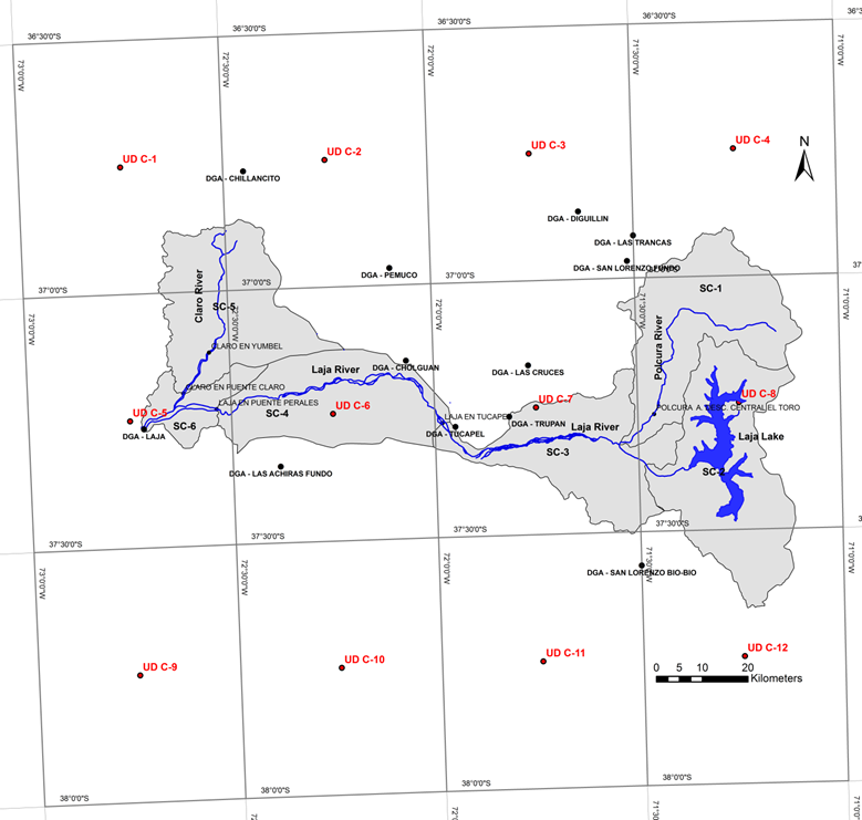
Figure 1 Study area. The sub-basins (SC) of the Laja River are shown in gray. The black dots indicate the meteorological stations, the gray dots streamflow stations and the red dots the centers of the quadrants with temperature records published by the University of Delaware. Lake Laja is shown in blue at the head of the basin and the blue lines indicate the primary water courses of the watershed, while the red arrows indicate anthropogenic alterations (canals) that extract or transfer water from each sub-basin.
The Laja River has a multi-use, snow-rain regime in which there is a complex interaction among the natural, economic and social components that control the use and management of resources (Muñoz, 2010).
In the lower half of the basin, there are 6 temperate-dry months and 6 cold-wet months (Mediterranean climate) on average. Annual precipitation ranges from 1,200 mm at its western border to over 1,500 mm in its eastern area. The temperature in the basin varies from 21ºC in the warmest month (January) to 8ºC in the coldest (July). In the Andes, there are notably different climatic zones according to the altitude. Above 500 masl, the temperature decreases and precipitation amounts surpass 2,300 mm/year. In the Lake Laja area, the average annual temperature is less than 10ºC, varying between average monthly temperatures of approximately 6ºC in July and 15 ºC in January. In the high cordillera, from 1,500 to 2,000 masl, a high-altitude cold climate predominates. The average snow line is above 2,600 masl, which explains why the presence of glaciers is limited to the highest peaks in the watersheds, located on Sierra Velluda (Mardones & Vargas, 2005).
The basin presents seasonal and interannual variability (Muñoz, 2011). The former is related to the location of the basin (in a temperate zone), while the latter is associated with climatic phenomena such as El Niño Southern Oscillation (ENSO).
There is an orographic effect in the cordillera zone that results in increased precipitation with strong precipitation gradients, as well as a sharp decrease in temperature resulting from high thermal gradients of up to -7 ºC/1000 m (DGA, 1983).
Figure 1 shows the Laja River basin, which for the present study was broken into six sub-basins (from SC-1 upstream to SC-6 downstream). Due to the absence of streamflow records in a common period, SC-5 and SC-6 are not included in the present analysis. The main characteristics and anthropogenic alterations to each studied sub-basin are described below.
Polcura (SC-1)
A snow-rain watershed in which the streamflow produced is divided between two outlets, one that flows to SC-3 and is monitored by the Polcura Antes Descarga Central El Toro gauging station and another that flows to Lake Laja via the Alto Polcura Canal (SC-2).
Lake Laja (SC-2)
The Lake Laja watershed is located on a western slope of the Andes. It generates streamflows that discharge into SC-4. One outflow is produced by natural leakages from the lake, whose streamflow depends on the lake level, while the other is produced by the El Toro hydroelectric plant, which discharges downstream of the Polcura Antes Descarga Central El Toro station.
Upper Laja (SC-3)
This sub-basin receives three inputs (from the El Toro plant, leakages from Lake Laja and the discharge of SC-1) and has eight extractions (the Zañartu, Collao, Mirrihue, El Litre, Bulnes, Ortiz, Laja-Diguillín and Laja Sur canals). Five of these canals present streamflow records, and the streamflow extracted by the three remaining canals (the Zañartu, Collao and Mirrihue) can be estimated at 22% of the total. The streamflows in this sub-basin are monitored by the “Laja en Tucapel station,” which also separates the upper and lower parts of the Laja River.
Middle Laja (SC-4)
This sub-basin can be modeled as a watershed with a rainfall regime that receives streamflows from SC-3 and discharges into SC-6. The “Laja en Puente Perales” station is located at its outlet.
The modeling requires precipitation, temperature and potential evapotranspiration series, in addition to the morphological characterization of the basin; the latter was achieved through 1-arc-second resolution ASTER images. Precipitation series from the rain gauge stations near each sub-basin (see Table 1) (managed by the General Water Directorate (Dirección General de Aguas, DGA) and temperature series published by the University of Delaware (UD) Center for Climate Research (Willmott & Matsuura, 2009) were also used for the modeling.
Table 1 Description of the model parameters and input modification factors for the pluvial and snowmelt modules.
| Parameter | Description | Influence | |
|---|---|---|---|
| RAINFALL | Cmax | - Maximum runoff coefficient when sub-surface storage is saturated. | - EI |
| PLim [mm] | - Precipitation amount above which there is direct deep percolation (PPD). | - PPD | |
| D | - Percentage of precipitation above PLim that becomes PPD. | - PPD | |
| Hmax [mm] | - Maximum storage capacity in the sub-superficial layer. | - Cmax and ER | |
| PORC | - Fraction of Hmax that defines the water content in the soil below which there are restrictions on evaporation processes. | - Hcrit and ER | |
| Ck | - Underground runoff coefficient. | - ES | |
| A | - Precipitation data adjustment factor. | - PM | |
| B | - Evapotranspiration data adjustment factor. | - PET and ER | |
| SNOWMELT | M [mm °C-1] | - Fraction of snow that melts above a base temperature (Tb) of snowmelt initiation. | - PSP, PS |
| Tb [°C-1] | - Base temperature that indicates the initiation of snowmelt (normally 0 °C). | - PSP, PS | |
| DM | - Minimum snowmelt rate when Tm < Tb. | - PSP, PS | |
| F | - Percentage of melted snow that is incorporated into direct runoff. | - DR | |
| FgT | - Thermal gradient data adjustment factor (should be 1 if the thermal gradient is measured in the field). | - Pnival | |
Potential evapotranspiration was calculated using the Thornthwaite method and the UD temperature data series. The spatial distribution of these variables over each sub-basin was calculated using Thiessen polygons.
Due to the availability and quality of the input data, the model was developed at a monthly time step for the analysis period of 1990 to 2002. The streamflow monitoring stations used were “Polcura antes Descarga Central El Toro” (SC-1), “Laja en Tucapel” (SC-3) and “Laja en Puente Perales” (SC-4). The Lake Laja watershed (SC-2) was not modeled because of lack of knowledge about the rules of operation of the El Toro hydroelectric plant and the lake volume-surface area relationships as a function of its level, information which is necessary for modeling.
Semi-distributed Muñoz Hydrological Model (MHM)
In this study, the semi-distributed rain-snow water balance model presented in Muñoz (2010) and Muñoz, Rivera, Vergara, Tume and Arumí (2014) was used (see conceptual diagram in Figure 2). This model simulates rainfall and snowmelt processes separately and allows anthropogenic alterations to the streamflow regime to be included by adding or subtracting flows.
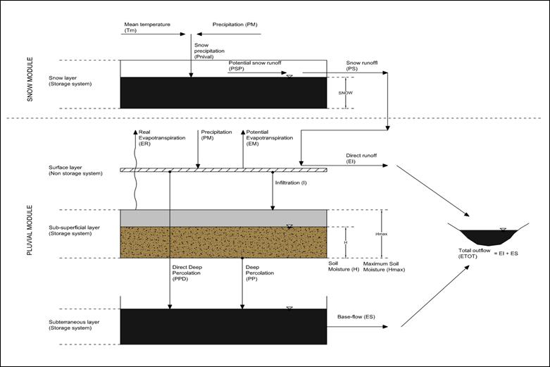
The rainfall component is modeled using a rainfall-runoff model that treats the watershed as a double storage system, with a sub-surface storage (SS) system and an underground storage (US) system. SS represents the water stored as soil moisture in the unsaturated soil layer. US represents the water stored in the saturated soil layer. The model requires two inputs: precipitation (P) and potential evapotranspiration (PET). The model output is total runoff (ETOT) at the watershed outlet, which is composed of underground runoff (ES) and direct runoff (EI). The runoff amounts are calculated using six calibration parameters and two that allow the input variables to be modified (necessary in cases in which P and PET are not representative of the watershed).
The snowmelt component determines snowfall (Pnival) based on precipitation above the 0 (°C) isotherm. Pnival is stored in the snow storage system (SN), which is used for the snowmelt calculations based on the concept of the degree-day method (Rango & Martinec, 1995). Using this method, the potential snowmelt (PSP) is calculated, and then based on the snow stored, the actual snowmelt (PS) is determined. Then PS is distributed in the rainfall model through a calibration parameter. Table 1 presents a brief description of the parameters and their influence on the model.
Finally, the model contains an anthropogenic alteration module that allows for changes that affect the streamflow regime to be incorporated into the model, such as changes in canals or industrial activities. It simulates the input to and/or outputs of a watershed via the addition or subtraction of flows (Eq. 1)
where the watershed discharge (Qoutput) on the time step t is equivalent to the watershed runoff (ETOT) plus the input streamflows (Qinputs) minus extractions (Qextractions) during the same period.
Methods
Calibration, uncertainty analysis and propagation
To carry out the calibration and uncertainty analysis process, the Monte-Carlo Analysis Toolbox (MCAT) was used. MCAT allows the identifiability of a model and its parameters and their relationship to its outputs to be investigated (Wagener, Lees, & Wheater, 2004).
Identifiability is defined as the influence of the values of a model parameter on its results, or the relationship between them. From here, positive identifiability refers to connections or relationships that make it possible to identify the simulated parameters and processes that positively influence the model results. Meanwhile, negative identifiability corresponds to relationships that negatively affect the model outputs.
To evaluate identifiability and quantify the uncertainty of a model, MCAT operates by running repeated simulations using a set of randomly-selected parameters within a user-defined range. The program stores the outputs and values of the defined objective function(s) for subsequent assessment of model behavior.
The parameters of hydrological models typically cannot be identified with a unique set of values (Muñoz et al., 2014), as different values of the same parameter set or even different models can represent equivalent results or solutions (equifinality) (Beven & Freer, 2001). This is due to the fact that changes in one parameter can be compensated for by changes in another or others due to their interdependence (Bárdossy, 2007). As a result of this interconnection among calibration parameters, an iterative process must be carried out for calibration, delimiting the range of identifiable parameters in order to observe identifiability in the remaining parameters (Muñoz et al., 2014).
For the model calibration, 15,000 simulations were run using sets of parameters that were randomly selected from a range defined according to their conceptual representation and based on prior experiences with the model (e.g., Ortiz, Muñoz, & Tume, 2011; Zúñiga, Muñoz, & Arumí, 2012). Each set is made up of 13 parameters, 8 associated with rainfall-runoff processes and 5 with snow accumulation and melting processes (Table 1).
The calibration process consisted of restricting the model parameter range through a positive and negative identifiability analysis. To this end, a cumulative distribution function of each parameter was graphed for the best 10% (positive identifiability) and worst 10% (negative identifiability) of the models, according to the objective function used. Based on the results of the identifiability analysis, the variation range of each parameter was delimited in order to subsequently repeat the analysis (performing 15,000 simulations along with a new identifiability analysis). This procedure was repeated until no identifiable parameters were observed.
As an example, Figure 3 shows an identifiability graph for parameter A, in which the magenta curve shows the cumulative distribution function (CDF) for the best 10% of the simulations and the cyan line shows the CDF for worst 10% of the solutions. From this figure it can be established that the best models are grouped in the range of A between 1.0 and 1.4, and therefore based on positive identifiability the range in which A positively identifies the results can be defined. In contrast, using negative identifiability (in cases in which positive identifiability is not observed), the range in which A is repeated most frequently in the worst obtained models (e.g., range of A between 2.1 and 2.5) can be discarded.
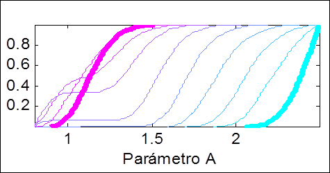
Figure 3 Example of identifiability analysis of parameter A using the KGE objective function for SC-1. The graph shows the CDF associated with 10% simulation groups, from the worst 10% of the models (cyan) to the best 10% of the models (magenta).
As a result of the identifiability analysis, a combination of possible results is obtained, and therefore there is uncertainty in the outputs (results) of the model. This uncertainty (associated with the model structure and parameters) was determined according to the Generalized Likelihood Uncertainty Estimation (GLUE) method described by Beven & Binley (1992) and Beven & Freer (2001).
With calibration parameter and model structure uncertainty defined, the effect of uncertainty in the input variables on the model results was quantified and its propagation downstream was analyzed. To this end, the model inputs (precipitation) in different periods and magnitudes were modified (in accord with the indications in Table 2) and the average ranges of the uncertainty bands of the model outputs were calculated. In this stage, to calculate the uncertainty in the outputs, 15,000 simulations were run with the previously-defined parameter ranges and precipitation that varied randomly for each simulation, but which was within the ranges and seasons indicated in Table 2. Then, based on the obtained results and following the GLUE method, the uncertainty bands of the model results were calculated again. In this case, the uncertainty bands include the structural and parametric uncertainty of the model plus the uncertainty associated with precipitation variation.
Table 2 Percentage change in precipitation in different time periods.
| Change period | Change (%) | ||||
|---|---|---|---|---|---|
| Entire year (Jan. - Dec.) | ±5 | ±10 | ±15 | ±20 | ±25 |
| Winter (Jun. - Aug.) | ±5 | ±10 | ±15 | ±20 | ±25 |
| Summer (Dec. - Feb.) | ±5 | ±10 | ±15 | ±20 | ±25 |
| Basin recharge (Apr. - Jun.) | ±5 | ±10 | ±15 | ±20 | ±25 |
| Basin drainage (Sep. - Nov.) | ±5 | ±10 | ±15 | ±20 | ±25 |
The Kling-Gupta efficiency (KGE; Gupta, Kling, Yilmaz, & Martinez, 2009) objective function (Eq. 2) was used for this analysis,. The KGE function is an improvement of the Nash-Sutcliffe efficiency index (NSE) (Nash & Sutcliffe, 1970), in which the correlation, deviation and variability components are equally weighted, resolving systematic problems of underestimation of maximum values and low variability identified in the NSE function (Gupta et al., 2009). KGE varies from -∞ to 1, where a value closer to 1 indicates that the model is more precise Eq. 2).
Results and discussion
Table 3 presents the calibration stage results. This shows the ranges obtained from the identifiability analysis for each analyzed sub-basin and the KGE values for the best model obtained according to the indicated ranges. The KGE values indicate that models rated “very good” are obtained in the three modeled sub-basins. In addition, it is observed that the ranges associated with the snowmelt component of the model were not delimited, which is in keeping with the insensitivity of the model to snowmelt processes in SC-1. Then, using the ranges obtained for each parameter and sub-basin (Table 3) and the GLUE method, the initial uncertainty of the model was estimated (Figure 4), and on this basis the influence of precipitation on uncertainty in the outputs was estimated.
Table 3 Final model parameter ranges obtained from identifiability analysis and KGE values of the best simulated model for each sub-basin.
| RAINFALL MODEL | ||||
|---|---|---|---|---|
| Sub-basin | SC-1 | SC-2 | SC-3 | SC-4 |
| Cmax | 0.31 - 0.32 | - | 0.289 - 0.294 | 0.288 - 0.300 |
| Hmax | 165 - 167 | - | 225 - 250 | 395 - 420 |
| D[%] | 0.1 - 0.6 | - | 0.42 - 0.50 | 0.55 - 0.60 |
| Plim[mm] | 200 - 1000 | - | 100 - 150 | 73 - 85 |
| PORC[%] | 20 - 37 | - | 40 - 60 | 20 - 32 |
| Ck | 0.33 - 0.34 | - | 0.276 - 0.280 | 0.215 - 0.230 |
| SNOWMELT MODEL | ||||
| M [mm°C-1] | 1 - 12 | - | - | - |
| Tb [°C] | 0 | - | - | - |
| DM | 0.1 - 0.6 | - | - | - |
| F | 0 - 1 | - | - | - |
| MASS BALANCE | ||||
| A | 1.19 | - | 1.53 | 1 |
| B | 1 | - | 1 | 1 |
| FgT | 1.58 | - | - | - |
| KGE | 0.90 | - | 0.93 | 0.94 |
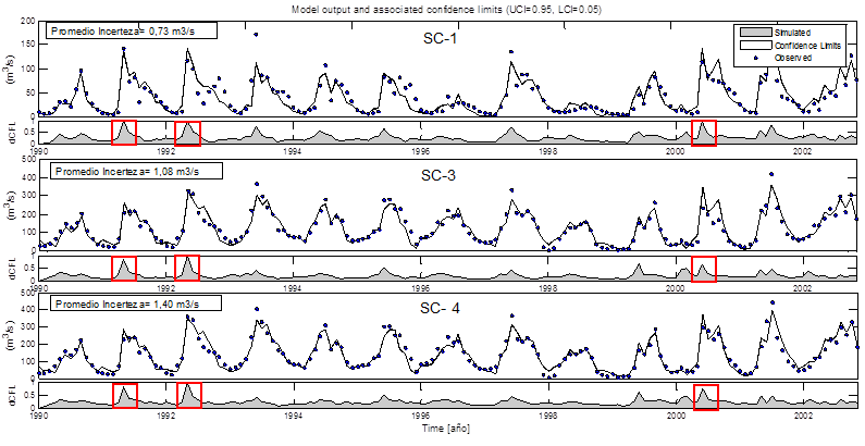
Figure 4 Uncertainty in hydrological model outputs for the three analyzed sub-basins. Each figure presents two boxes. The upper box shows the uncertainty band associated with the model and its parameterization along with the recorded streamflows. The lower box shows the relative and normalized uncertainty. The red squares indicate the periods of greatest uncertainty in each sub-basin.
Figure 4 shows that the model offers a good approximation for SC-1, SC-3 and SC-4 in terms of the observed streamflows. In addition, it is observed that the temporal distribution of uncertainty varies, and is greater in winter than in summer (see relative uncertainty over time and red squares in Figure 4). Similarly, it is observed that relative uncertainty is maintained downstream, and is greater in the same periods in the three sub-basins. This suggests either that the propagation of uncertainty is dependent on or sensitive to uncertainty upstream or that the model tends to be more sensitive in the aforementioned periods and therefore has greater uncertainty in streamflow estimation during high-water periods.
Figure 5 shows the influence of variation (or uncertainty) in precipitation depending on the season or period of the year, and how it propagates downstream in the model. A proportional relationship can be seen between the magnitude of variation (or uncertainty) in precipitation and the uncertainty in the model results. Similar results are observed for uncertainties in precipitation during periods in which rainfall is concentrated (watershed recharge periods and winter). In addition, uncertainty in the outputs is relatively independent of the uncertainty in precipitation during summer and drainage periods. This suggests that the magnitude of precipitation during these periods is insufficient to affect the streamflows of the basin and therefore these streamflows depend mainly on the basin storage status more than the magnitude of precipitation that occurs during the period. This result suggests an advantage for streamflow estimation during low-water periods and water planning during irrigation seasons. In this case, it is more convenient to appropriately estimate the basin conditions prior to the low-water season than, for example, forecasting precipitation amounts in the coming months. Meanwhile, if streamflows are to be measured during basin recharge or rainy periods (between April and August), appropriately measuring and forecasting rainfall amounts in the basins studied is crucial given that, depending on the watershed characteristics, there is an uncertainty of up to nearly 20% in streamflows for an uncertainty of 25% in precipitation.
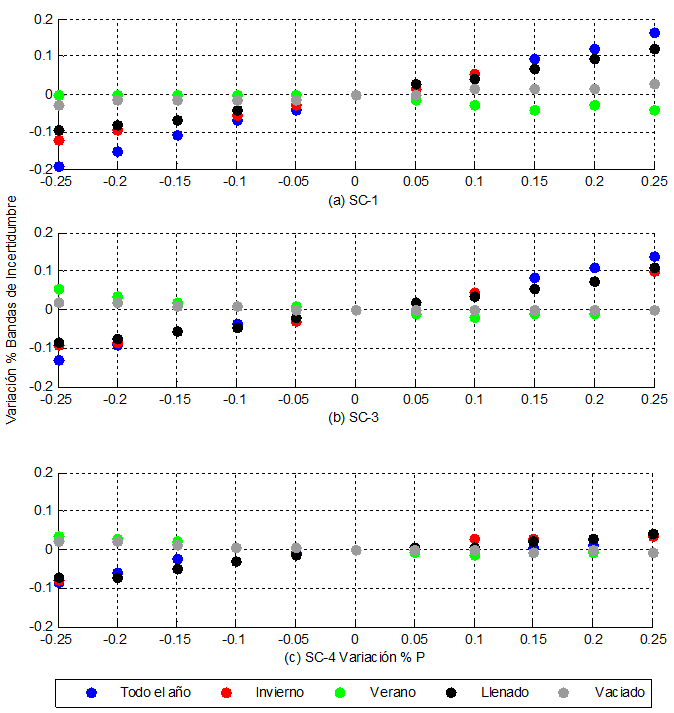
Figure 5 Percentage change in average uncertainty bandwidth of the hydrological model outputs for each sub-basin as a function of uncertainty in precipitation.
Regarding the propagation of uncertainty, influence downstream could be assumed (Figure 4); however, relative uncertainty and the percentage change in the uncertainty bands decrease downstream (Figure 5). This suggests that there is no propagation of uncertainty downstream, but rather, the uncertainty of the results is associated with the magnitude of the modeled streamflows more than the effects of propagation downstream.
Figure 6 presents the seasonal variability of the simulated streamflows for the base condition for changes in precipitation of ±25% and the different studied periods. As can be seen, for variations in precipitation over the course of the year, the months with the greatest output variability, and which are therefore the most influential on the model outputs, are May, June, July, August and September, with streamflow differences in the median of the boxplots of approximately 25 m3/s (in comparison with the initial uncertainty of the model). In addition, a larger range of simulated streamflows is observed during the rainy months for the entire year and forwinter and basin recharge periods for SC-1, SC-3 and SC-4. The opposite effect occurs for negative uncertainty in precipitation, with the amplitude of the boxplots decreasing, bringing the quartile boundaries closer to the median for rainy periods, which reflects a decrease in high streamflows, exhibiting a high sensitivity to them. This is evident as the 3rd quartile decreases more than the 1st. The boxplots in Figure 6 confirm the results observed in Figure 5 regarding a greater influence on the model outputs during rainy periods and the relative independence of the model with respect to the uncertainty in during drainage and summer periods.
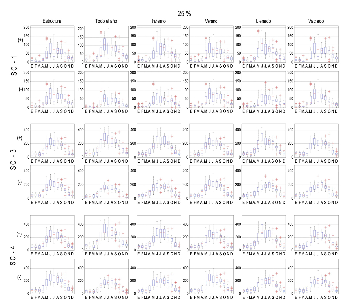
Figure 6 Boxplots of the model streamflow for the simulated period as a function of a positive or negative percentage change in precipitation of 25% (keeping fixed model uncertainty, i.e., structure and parameterization). The x axis shows the months of the year and the y axis shows the simulated streamflows in m3/s.
Conclusions
The effect of uncertainty in precipitation on the streamflow estimation of a semi-distributed hydrological model was analyzed and quantified. As a result, uncertainty in precipitation during periods in which it is concentrated (winter) was found to have a proportional effect on the outputs (streamflows) of a hydrological model. Meanwhile, during the summer, uncertainty in model outputs is insensitive to precipitation variations that occur during the same period. Therefore, if predictive models are to be constructed, according to the use of each, then critical points to address must be defined in order to delimit the uncertainty of a hydrological model. If a model for irrigation is required, the storage conditions of the basin need to be appropriately estimated since uncertainty in precipitation in the summer does not greatly affect uncertainty in the model outputs. In addition, if a model is required for streamflow forecasting in winter or for reservoir management, an accurate estimation of precipitation is essential, as is the determination of the uncertainty associated with this variable. Otherwise, this uncertainty would almost completely convert to uncertainty in the streamflows estimated by the model.
From the analysis of the downstream propagation of uncertainty in the results of the semi-distributed model used, the magnitude of the simulated streamflows was found to have a greater incidence than the propagation of uncertainty. Therefore, the correct measurement and estimation of precipitation in the basin, or the correct estimation of its storage level (according to the purpose of the modeling), takes on even greater importance.
Acknowledgments
The authors are grateful to the Dirección General de Aguas for providing the precipitation and streamflow data and FONDECYT Project 11121287, “Hydrological process dynamics in Andean basins. Identifying the driving forces and implications in model predictability and climate change impact studies,” which supported the development of this research.
REFERENCES
Bárdossy, A. (2007). Calibration of hydrological model parameters for ungauged catchments. Hydrology and Earth System Sciences, 11(2), 703-710. [ Links ]
Beven, K., & Binley, A. (1992). The future of distributed models: Model calibration and uncertainty prediction. Hydrological Processes, 6, 279-298. [ Links ]
Beven, K., & Freer, J. (2001). Equifinality, data assimilation, and uncertainty estimation in mechanistic modelling of complex environmental systems. Journal of Hydrology, 249, 11-29. [ Links ]
Butts, M., Paynea, T., Kristensenb, M., & Madsen, H. (2004). An evaluation of the impact of model structure on hydrological modelling uncertainty for streamflow simulation. Journal of Hydrology, 298, 242-266. [ Links ]
Deletic, A., Dotto, C., McCarthy, D., Kleidorfer, M., Freni, G., Mannina, G. et al. (2012). Assessing uncertainties in urban drainage models. Physics and Chemistry of the Earth, 42-44, 3-10. [ Links ]
Dirección General de Aguas, DGA. (1983). Balance Hidrológico Nacional Regiones VIII, IX y X. México, DF: Dirección General de Aguas. [ Links ]
Dirección General de Aguas, DGA. (2013). Sendas del agua. Desafíos de la Nueva Estrategia Nacional de Recursos Hídricos. Recuperado de http://www.dga.cl/Documents/Sendasdelagua012013.pdf [ Links ]
Fekete, B., Vörosmarty, C., Roads, J., & Willmott, C. (2004). Uncertainties in precipitation and their impacts on runoff estimates. Journal of Climate, 17, 294-304. [ Links ]
Gattke, C., & Schaumann, A. (2007). Comparison of different approaches to quantify the reliability of hydrological simulations. Advances in Geoscience, 6, 15-20. [ Links ]
Gupta, H., Kling, H., Yilmaz, K., & Martinez, G. (2009). Decomposition of the mean squared error and NSE performance criteria: Implications for improving hydrological modeling. Journal of Hydrology, 377, 80-91. [ Links ]
Grupo Intergubernamental sobre Cambio Climático, IPCC. (2007). Informe del Grupo Intergubernamental de Expertos sobre el Cambio Climático. Recuperado de https://www.ipcc.ch/pdf/assessment-report/ar4/syr/ar4_syr_sp.pdf [ Links ]
Grupo Intergubernamental sobre Cambio Climático, IPCC. (2013). Intergovernmental Panel on Climate Change. Recuperado de http://www.climatechange2013.org/images/uploads/WGIAR5_WGI12Doc2b_FinalDraft_All.pdf [ Links ]
Mardones, M., & Vargas, J. (2005). Efectos hidrológicos de los usos eléctricos y agrícolas en la cuenca del río Laja (Chile Centro-Sur). Revista de Geografía Norte Grande, 33, 89-102. [ Links ]
McMillan, H., Krueger, T., & Freer, J. (2012). Benchmarking observational uncertainties for hydrology: Rainfall, river discharge and water quality. Hydrological Processes, 26, 4078-4111. [ Links ]
Muñoz, E. (2010). Desarrollo de un modelo hidrológico como herramienta de apoyo para la gestión del agua. Aplicación a la cuenca del Río Laja, Chile (tesis de maestría). Universidad de Cantabria, Escuela de Caminos Canales y Puertos, Santander, España. [ Links ]
Muñoz, E. (2011). Perfeccionamiento de un modelo hidrológico aplicación de análisis de identificabilidad dinámico y uso de datos grillados (tesis de doctorado). Departamento de Recursos Hídricos, Universidad de Concepción, Chillán, Chile. [ Links ]
Muñoz, E., Álvarez, C., Billib, M., Arumí, J. L. & Rivera, D. (2011). Comparison of gridded and measured rainfall data for hydrological studies at basin scale. Chilean Journal of Agricultural Research, 71(3), 459-468. [ Links ]
Muñoz, E., Arumí, J. L., & Rivera, D. (2013). Watersheds are not static: Implications of climate variability and hydrologic dynamics in modeling. Bosque, 34(1), 7-11. [ Links ]
Muñoz, E., Rivera, D., Vergara, F., Tume, P., & Arumí, J. L. (2014). Identifiability analysis: Towards constrained equifinality and reduced uncertainty in a conceptual model. Hydrological Sciences Journal, 59(9), 1690-1703. [ Links ]
Nash, J., & Sutcliffe, J. (1970). River flow forecasting through conceptual models part I: A discussion of principles. Journal of Hydrology, 10(3), 282-290. [ Links ]
Ortiz, G., Muñoz, E., & Tume, P. (octubre, 2011). Incerteza en las variables de entrada de un modelo hidrológico conceptual. Efectos sobre la incerteza en las salidas. XX Congreso Chileno de Hidráulica. Congreso llevo a cabo en Santiago, Chile. [ Links ]
Rango, A., & Martinec, J. (1995). Revisting the degree-day method for snowmelt computations. Journal of the American Water Resources Association, 31(4), 657-669. [ Links ]
Shen, Z., Chen, L., & Chen, T. (2012). Analysis of parameter uncertainty in hydrological and sediment modeling using GLUE method: A case study of SWAT model applied to Three Gorges Reservoir Region, China. Hydrology and Earth System Sciences, 16, 121-132. [ Links ]
Wagener, T., Lees, M., & Wheater, H. (2004). Monte-Carlo analysis toolbox user manual. Recuperado de http://www3.imperial.acuk/ewre/research/software/toolkit [ Links ]
Westerberg, I., & McMillan, H. (2015). Uncertainty in hydrological signatures. Hydrology and Earth System Sciences, 19(9), 3951-3968. [ Links ]
Willmott, C., & Matsuura, K. (2009). Terrestrial air temperature and precipitation: Monthly and annual time series (1900-2008). Version 3.01. Recuperado de http://climate.geog.udel.edu/climate [ Links ]
Zúñiga, R., Muñoz, E., & Arumí, J. (2012). Estudio de los procesos hidrológicos de la cuenca del río Diguillín. Obras y Proyectos, 11, 69-78. [ Links ]
Received: May 16, 2016; Accepted: October 24, 2017
 Este es un artículo publicado en acceso abierto bajo una licencia
Creative Commons
Este es un artículo publicado en acceso abierto bajo una licencia
Creative Commons
