Introduction

^{Pollak (2012)} considered that mathematicians usually divide the universe between mathematics, and the rest of the world, but the truth is that mathematics is needed to understand a situation in the real world, and then maybe to be used to take action or sometimes to forecast the future. It does not matter if the problem is important or not, the real world and mathematics have to be taken seriously. The relationship between mathematics and the real world usually is the same. The situation in the real world is so diverse and complex that it is not possible to take everything into consideration, so it is necessary to simplify and decide which aspects are most important, that means we have an idealized version of a situation in the real world, a system, which then can be translated into mathematical terms, this entire process is called mathematical modeling (^{Pollak, 2012}).

^{Eykhoff (1974)} considered that a mathematical model is the representation of the most important aspects of a system, with enough knowledge of that system in usable form. Therefore, modeling is an activity representing how systems, objects or even nature behave under some theoretical assumptions. These systems can be described by words, drawings, sketches, physical models, computer programs, or mathematical formulas, therefore, the modeling activity can be done in several languages, usually simultaneously, and here we are focused in the physical and mathematical language to build models (^{Quarteroni, 2009}).

Figure 1 shows a simplified version of the modeling process from a problem to its solution applying the scientific method (^{Dym & Ivey, 1980}).

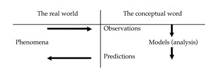
Figure 1 Simplified version of the modeling process from a problem to its solution applying the scientific method (^{Dym & Ivey, 1980}). 

In the other side, ^{Pollak (2012)} stated the difference between mathematical modeling and problem-solving. A problem solving may not refer to the outside world at all. Even when it does, problem-solving usually begins with the idealized situation in the real world in mathematical language, and finish with a mathematical solution or result. Mathematical modeling on the other hand, begins with a system and requires problem formulating before problem-solving, and once the problem is solved, moves back into the system where the results are considered in their original context (^{Pollak, 2012}).

For ^{Quarteroni (2009)}, mathematical modeling goal is to describe the different aspects of a system in the real world following the scientific method (figure 2), the interaction between observations, phenomena, predictions, and their dynamics through mathematics.

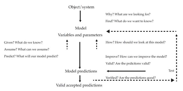
Figure 2 Interaction between observations, phenomena, predictions, and their dynamics through mathematics inspired by ^{Carson and Cobelli (2001)}. 

For ^{Carson and Cobelli (2001)} the necessary questions for a successful creation of a model are the following: Why? Identify the need for the model. Find? List the data we are seeking. Given? Identify the available relevant data. Assume? Identify the circumstances that apply. How? Identify the governing physical principles. Predict? Identify the equations that will be used, the calculations that will be made, and the answers that will result. Valid? Identify tests that can be made to validate the model and if the results are consistent with its principles and assumptions. Verified? Identify tests that can be made to verify the model.

Mathematical models (^{Quarteroni, 2009}) also offer new possibilities to manage the increase complexity of technology, which is at the basis of modern industrial production due that models can save time and money in the development and validation phases, besides that models can explore new solutions in a very short period.

Models can be distinguished by the reason for their application, it can be dynamic if it has changed over time or stationary/static if it does not. Models can vary from policy analytical to scientific research models, operational models for real-time control of structures, calamity models and also overlap field of studies. But a mathematical model must be able to address universal scientific concepts, and it is necessary to define which level of detail must be introduced in the different parts of a model (^{Quarteroni, 2009}).

Hydrology was defined by ^{Penman (1961)} as the science that attempts to answer the question: What happens to the rain? This could be a simple question, but experience has shown that quantitative descriptions of the land phase of the hydrologic cycle is very complicated and has a great deal of uncertainty. One-step forward to answer this question is the simplification of the hydrologic system, not just what happens with the rain in general, but what happens with the rain in a watershed. As ^{Zin (2002)} says, actual watershed theories cannot be generalized for all the processes and their interactions, due to the spatial and temporal heterogeneity of the watersheds.

Watershed hydrology is defined as the branch of hydrology that works with the hydrologic processes at the watershed scale to determine and understand the laws that rules the watershed (^{Singh & Woolhiser, 2002}). A watershed may be as small as a backyard or large with hundreds of thousands of square kilometers, therefore hydrologic processes and their spatial non uniformity are defined by climate, topography, geology, soils, vegetation, and land use and all of them are related to the size of the watershed (^{Singh & Woolhiser, 2002}), but due to the complexity and large variability of the watersheds, they cannot be globally described and studied; modelling is necessary to analyze and predict their dynamics (^{Zin, 2002}).

Watershed models are fundamental to water resources assessment, development, management, planning, design, and operation of projects, to conserve water and soil resources and to protect their quality and to understand dynamic interactions between climate and land-surface hydrology, for example, vegetation, snow cover, active permafrost layer, etc. are quite sensitive to the lower boundary of the atmospheric system (^{Singh & Woolhiser, 2002}). Also, they are used to analyze the quantity and quality of streamflow, reservoir system operations, groundwater development and environmental protection, surface water and groundwater management, water distribution systems (^{Wurbs, 1998}) and to quantify the impacts of watershed management strategies, linking human activities within the watershed to water quantity and quality of the receiving stream or lake (^{Rudra, Dickinson, Abedini, & Wall, 1999}), for environmental and water resource protection and the integration this watershed models with models of physical habitat, biological populations, and economic response (^{Singh & Woolhiser, 2002}; ^{Hickey & Diaz, 1999}).

Mathematical models for watershed hydrology are designed to answer Penman’s question at a level of detail depending on the problem and are employed in a wide field of areas, from watershed management and environmental protection to engineering design (^{Singh, 1995}). At the field scale, models are used for varied purposes, such as planning and designing soil conservation practices, irrigation water management, wetland restoration, stream restoration, and water-table management. On a large scale, simulation models are used for flood protection projects, rehabilitation of aging dams, floodplain management, water-quality evaluation, and water-supply forecasting (^{Singh & Woolhiser, 2002}), even though there is not a simple or universal solution to all modelling and simulation problems as ^{Van Waveren et al. (2000)} has taken us to attention.

^{Klemeš´s (1986)} opinion is that, at the present stage of hydrologic sciences, hydrologic modeling is most credible when it does not pretend to be too sophisticated and all-inclusive, and remains confined to those simple situations whose physics is relatively well understood. For ^{Kirchner (2006)}, advancing the science of hydrology will require new hydrologic measurements, new methods for analyzing hydrologic data, and new approaches to modeling hydrologic systems rather than models with a huge number of parameters, besides ^{Kirchner (2006)}, is not the first to mention such approach, other like ^{Klemeš (1986}, 1988); Grayson et al. (1992); and Beven (2002), they did before.

Some promising research directions in the study of hydrology, in ^{Kirchner´s (2006)} opinion, include (1) designing new data networks, field observations, and field experiments, recognizing the spatiotemporal heterogeneity of hydrologic processes, (2) developing gray box data analysis methods that are more compatible with the nonlinear and non-additive character of hydrologic systems, (3) developing physically based ruling equations for hydrologic process at hill/slope scale and understanding that they could look different from the equations that describe the small-scale physics, (4) developing models that are minimally parameterized, and therefore stand some chance of failing the tests that they are subjected to, (5) developing ways to test models more comprehensively and incisively (^{Kirchner, 2006}).

One type of mathematical models are the Black-Box models (^{Brooks, Folliott, Greggersen, & Thames, 1991}). These models are based solely on empirical relationships between one or more inputs and outputs. The internal processes in the system being modeled are unknown and not represented in the form of a conservation of mass, momentum or energy approach. Typically, the input-output relationships are based on statistics such as a regression equation. Frequently, the regression constants are given as coefficients with little or no information regarding the variability. Examples in the field of hydrology include the Rational Equation and the Unit Hydrograph (^{Brooks et al., 1991).} Another type of mathematical models commonly used in science and engineering is the physical or process-based model. In this type of models, the underlying relationships among inflows, storages and outflows are represented through physics and basic principles of conservation of mass, momentum and/or energy and can be classified as follows (^{Sjöberg et al., 1995}).

For Black-Box models (^{Sjöberg et al., 1995}) the area is quite diverse, and covers topics from mathematical approximation theory, via estimation theory and non-parametric regression, to algorithms and currently much-discussed concepts like neural networks, wavelets and fuzzy models . There are important links to classical statistical approaches in non-parametric regression and density estimation, with kernel methods and nearest-neighbor techniques such as Kung (1993), and Haykin (1994), fuzzy models, like Brown and Harris (1994) and Wang (1994), non-parametric regression and density estimation, like Stone (1982), Silverman (1986) and Devroye and Gyorfi (1985), and wavelets and multiresolution techniques, like Meyer (1990), Daubechies (1992) Chui (1992) and Ruskai et al. (1992).

The key problem in system identification for Black-Box modeling is to find a suitable model structure within which a good model is to be found. Fitting a model by parameter estimation is in most cases not difficult. A basic rule in estimation is not to estimate what you already know. In other words, one should utilize prior knowledge and physical insight about the system when selecting the model structure.

For ^{Sjöberg et al. (1995)} the problem we are addressing in this research related to the application of a Black-Box model in hydrology is how to infer relationships between past input-output data and present-future outputs of a system when very little a priori knowledge is available, this is known as Black-Box modeling. There is a rich and well-established theory for Black-Box modeling of linear systems (e.g., Ljung, 1987; Sderstrom & Stoica, 1989). It was not until the last few years that modeling and identification of nonlinear systems attracted wide interest in the control community. So far, almost all attention has been concentrated on one single structure-neural networks. However, nonlinear modeling has been studied for a long time in the statistics community, where it is known under the label non-parametric regression (^{Sjöberg et al., 1995}).

The task of Black-Box linear models has, is to describe the systems frequency response or impulse response, just a mapping the number of inputs and outputs, but the nonlinear Black-Box situation is much more difficult. The main reason is that nothing is excluded, and a very rich spectrum of possible model descriptions must be handled. In this document, we shall discuss the possibilities and limitations with such nonlinear Black-Boxidentification (^{Sjöberg et al., 1995}).

This paper describes the concepts and limitations of a Black-Box model as compared to a process-based model. The exercise starts with a physical Black-Box, known amounts of water are added to the vertical cylinder in the top of the box, while outflows are measured from the spout on one end, the two parameters inflow and outflow are then related statistically. Once the results of the Black-Box approach are completed, the top is removed from the box to reveal the internal structure and physical processes involved in the system. A process-based model is then constructed that includes the physics of flow based on the size and shape of the different storages and flow conveyances using Stella® (Systems Thinking, Experiential Learning Laboratory, with Animation) software to replicate the Black-Box model and develop a dynamic model to predict outflows for given inflows. This will help students to understand some of the limitations and uses of the mathematical and Black-Box models and understand some basic laws that rule the hydrologic.

Methods

Black-Box model

By definition a Black-Box model is a fitted mathematical representation of a system without regard to processes, the characteristics of such device usually are developed from observation of inputs/outputs, they don´t identify or simulate processes involved, usually they are statistically based, e.g. regression, and in hydrology, rainfall is input and runoff or discharge is output and as examples we can include the Rational equation and the Unit Hydrograph.

The Black-Box used for this experiment (figure 3), has a vertical input cylinder above the Black-Box that represents a vertical section of soil on which precipitation might fall as show figure 3a. Figure 3b shows a horizontal spigot with invert height of 7.5 cm permits runoff to occur to a second storage once the cylinder is filled to that height. This second storage represents a temporary pond or lake or wetland with a controlled outflow from the system via a V notch weir. Water can also exit the second storage as vertical flow through a small metal pipe to a third, enclosed storage that represents a groundwater aquifer. In this model, there is no groundwater discharge, however, one could easily be added. There is a slow discharge directly from the simulated soil cylinder to the groundwater storage through a small tube with an adjustable clamp to control the seepage rate from the soil, all this system is represented by the picture in figure 3b. The soil porosity and/or infiltration capacity can be changed by adding materials such as marbles with high or infiltration capacity or small glass beads with low or infiltration capacity. Figure 3c shows the application of a Black-Box simulation, throwing water over the vertical cylinder as representation of precipitation.

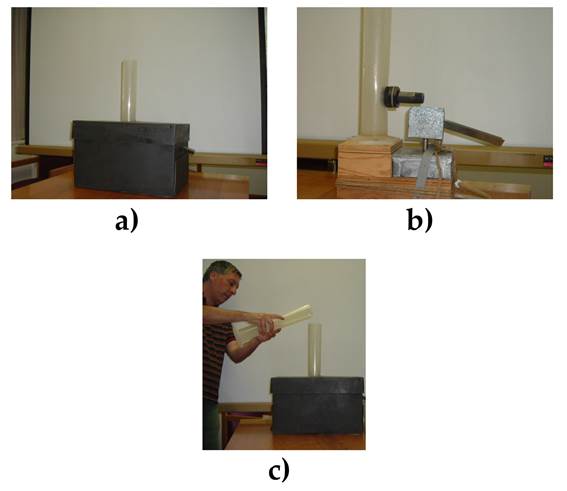
Figure 3 Photos of Physical Hydrologic Black-Box Model, a) External view of Black-Box, b) Internal components of the physical model with three reservoirs or storages, flow connectors from Soil to wetland and groundwater aquifer and c) Application of a Black-Box simulation throwing water over the vertical cylinder. 

Stella® Software model

Stella® software from ^{ISEE Systems Inc. (2003)} is an icon-based dynamic simulation software which permits the user to build dynamic models by connecting components in a diagram based on their concepts and ideas of how a system works. Equations that describe the conservation of mass, energy or momentum are automatically developed within Stella® as the icons for fluxes and storages are connected on the desktop. A user with limited programming skills can therefore easily build and run a model, and explore the influence of varied inputs and parameter values on the outputs. The icon-based software has boxes called stocks and are the storages of either mass or energy for a given reach of a stream, large arrows with valves represent fluxes of mass or energy into or out of the stock and the small thin arrows are connectors that indicate the dependence of one component another (Ford, 2000). The Stella® software automatically maintains conservation of mass based on the created diagram or flowchart, the mathematics of balance and conservation laws are straightforward at this level of abstraction and the solution to the underlying differential equations are solved by finite difference techniques behind the scenes with outputs in form of tables and graphs (Ford, 2000).

Figure 4 illustrates the Stella® diagram for the physical hydrologic Black-Box. The rectangles are stocks which represent the three different storages at a given instant of time. The pipe and valve icons are used to represent fluxes into or out of the storages; their units are volume per time. The circles are converters, which give parameter values or relationships between other components of the system in the form of equations or graphs. The arrows are connectors that the program uses to link the components. Built-in functions are readily available and conditional statements are easily incorporated.

Figure 4 Model of the Hydrologic Black-Box, illustrating the Stella® model diagram. 

The ruling equations to represent the Black-Box model using Stella® software are the standard hydraulic equations (^{Chow, 1964}) for the size and shape of the different pipes, storages and flow conveyances.

Velocity:

v=qA (1)

Where:

v	Average velocity (cm/s)
q	Flow rate (cm3/s)
A	Surface area (cm2)

Reynolds number:

Re=4*Vk*Rv (2)

Where:

Re	Reynolds number (-)
v	Average velocity (cm/s)
Vk	Kinematic velocitye (cm2/s)
R	Hydraulic radius (cm)

Energy Equation:

p1γ+z1+v122*g+Hg=p2γ+z2+v222*g+Hl (3)

Where:

p	Pressure (Kg/cm2)
γ	Specific weight (Kg/cm3)
z	Elevation (cm)
v	Fluid Velocity (cm/s)
g	Gravitational acceleration (cm/s2)
Hg	Head gain (cm)
Hl	Combined head loss (cm)

V notch weir:

q=815*2*g*tnθH232 (4)

Where:

q	Discharge (cm3/s)
θ	Angle (degrees)
C	Coefficient of discharge (-)
H	Head (cm)
R	Hydraulic radius (cm)

The model was calibrated to determine the best values of coefficients (e.g. orifice coefficients and friction factor) to use in the model (table 1). This parameter evaluation step is a necessity in all mathematical models and illustrates the value in coupling measurements of the physical system with mathematical modeling.

Table 1 Parameters of the Hydrologic Black-Box model applied with Stella®. 

Name	Units	Value
Inflow Cylinder Diameter	cm	6.25
Outlet Elevation	cm	10
Pipe diameter	cm	2.54
Orifice coefficient	-	0.8
Pan diameter	cm	10
V notch weir outflow angle	degrees	90
Invert elevation	cm	2
Small Drain Friction factor	-	0.1
Small Drain tube diameter	cm	0.5
Small Drain tube length	cm	50
Drainage pipe diameter	cm	1.25
Drainage pipe depth	cm	5
Subpan diameter	cm	12.5
Soil porosity	Percent	0.05
Reynolds number	-	1603

Results and discussion

Three simulated storms were applied to the Black-Box (table 2) of 75, 40 and 30 cm³/s separated by short intervals, and the outflows for the three storms were 2, 10 and 11 cm³/s, respectively.

Latter two more storms were added of 20 and 50 cm³/s separated by short intervals, and the outflows for the two storms were 19 and 45 cm³/s, respectively (table 3).

Figure 5 shows results of the Stella® Model in the form of rates of inflow versus V notch weir outflow.

Figure 5 Results of the inflows and simulated V notch weir outflow from the Stella® model. 

Figure 6 shows results of the Stella® Model in the form of rates of inflow versus outflow (figure 6a) and adding two more storms of 20 and 50 cm³/s with outflows of 19 and 45 cm³/s, respectively (figure 6b).

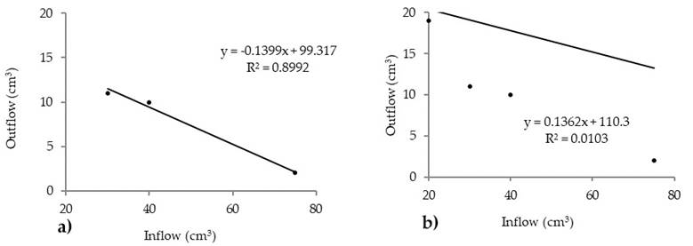
Figure 6 Results of Storms applied to Physical Black-Box Model, a) for three initial storms and b) for the total five storms. 

The good fit between the inflow and outflow is shown by the high Square-R of 0.89 were the total volume of inflow versus total volume of outflow values predicted by the model are similar to the measured values for the different storms. However, critical analysis of the relationship reveals a logic error. Outflow decreases as inflow increases, in contrast to the established, logical relationship. Acquisition of additional data by applying more storms reveals that the three initial points, although physically and empirically correct, only represent a small part of the complex relationships between inflow and outflow. It is clear that the Black-Box model cannot accurately predict inflow-outflow relationships without much more data, including additional parameters such as the initial conditions at the start of a storm.

Conclusions

Black-Box models are limited due to their inability to model basic governing processes such as conservation of mass and momentum in a system. Process-based models help in the analysis of a system under varied initial and boundary conditions. The combination of physical measurements and a process-based mathematical model such as Stella® could help students to understand some of the limitations and uses of each approach. An understanding of the basic laws that rule the hydrologic processes in a system is usually critical to the proper modeling and prediction of results under a variety of initial and boundary conditions. The typical Black-Box type of model is inherently limited due to a lack of understanding of the governing processes and inability to assess initial conditions which can lead to erroneous conclusions.